Research Article |
|
Corresponding author: Hans S. Reip ( reip@myriapoden-info.de ) Academic editor: Pavel Stoev
© 2018 Hans S. Reip, Thomas Wesener.
This is an open access article distributed under the terms of the Creative Commons Attribution License (CC BY 4.0), which permits unrestricted use, distribution, and reproduction in any medium, provided the original author and source are credited.
Citation:
Reip HS, Wesener T (2018) Intraspecific variation and phylogeography of the millipede model organism, the Black Pill Millipede Glomeris marginata (Villers, 1789) (Diplopoda, Glomerida, Glomeridae). In: Stoev P, Edgecombe GD (Eds) Proceedings of the 17th International Congress of Myriapodology, Krabi, Thailand. ZooKeys 741: 93-131. https://doi.org/10.3897/zookeys.741.21917
|
Abstract
The Black Pill Millipede, Glomeris marginata, is the best studied millipede species and a model organism for Diplopoda. Glomeris marginata is widespread, with numerous colour morphs occurring across its range, especially in the south. This study investigates whether colour morphs might represent cryptic species as well as the haplotype diversity and biogeography of G. marginata. The results of the COI barcoding fragment analysis include 97 G. marginata, as well as 21 specimens from seven potentially related species: G. intermedia Latzel, 1884, G. klugii Brandt, 1833 (G. undulata C.L. Koch, 1844), G. connexa Koch, 1847, G. hexasticha Brandt, 1833, G. maerens Attems, 1927, G. annulata Brandt, 1833 and G. apuana Verhoeff, 1911. The majority of the barcoding data was obtained through the German Barcode of Life project (GBOL). Interspecifically, G. marginata is separated from its congeners by a minimum uncorrected genetic distance of 12.9 %, confirming its monophyly. Uncorrected intraspecific distances of G. marginata are comparable to those of other widespread Glomeris species, varying between 0–4.7%, with the largest genetic distances (>2.5 %) found at the Mediterranean coast. 97 sampled specimens of G. marginata yielded 47 different haplotypes, with identical haplotypes occurring at large distances from one another, and different haplotypes being present in populations occurring in close proximity. The highest number of haplotypes was found in the best-sampled area, western Germany. The English haplotype is identical to northern Spain; specimens from southern Spain are closer to French Mediterranean specimens. Analyses (CHAO1) show that approximately 400 different haplotypes can be expected in G. marginata. To cover all haplotypes, it is projected that up to 6,000 specimens would need to be sequenced, highlighting the impossibility of covering the whole genetic diversity in barcoding attempts of immobile soil arthropod species.
Keywords
biogeographic regions, COI, Europe, haplotype analysis, haplotype richness estimation
Introduction
In recent decades the Black Pill Millipede, G. marginata (Glomerida, Glomeridae) has become a model organism of the Diplopoda. The Black Pill Millipede is morphologically the best studied species of the millipedes (see examples in
After discovering a new chemical compound in G. marginata (Glomerin:
The unusual mating behaviour of pill millipedes (involving the sperm ejaculation on a piece of soil before the transfer to the female) was studied extensively in the Black Pill Millipede (e.g.,
Glomeris marginata is commonly included in arthropod phylogenetic analyses (e.g., Regier 2001, 2005). The Black Pill Millipede is the only species of the Diplopoda in which gene expressions of different genes, including Hox genes, were widely researched (e.g.,
Despite the high importance of G. marginata for general studies of millipedes, and arthropod segmentation patterns in general, little to no taxonomic studies or population genetic studies of the species were conducted in recent decades. Recent genetic studies in congeneric pill millipedes allowed the detection of several synonymies as well as cryptic species, and clarified the taxonomic status of several Glomeris species (Hoess and Scholl 1999, 2001,
The lack of taxonomic studies in G. marginata is even more surprising considering the unusual wide distribution of the species (
While adult G. marginata normally can be easily distinguished from their congeners by their shiny completely black-brown colour with brightly coloured creamy-white tergal margins (see

Glomeris marginata (Villers, 1789) colour morphs. A main coloration form, center immature specimens showing the perplexa colour pattern; Germany, Landskrone B strongly lightened adult perplexa pattern, France, Pays de la Loire C red mutant, Germany, Bonn D strongly red-banded form, from France, Montauroux E more weakly red-brown banded from, France, same population as D. A, D, E photographed by Jan Philip Oeyen B by

A G. marginata, brown and black form occurring in sympatry, Germany, Rügen, 2016. B–G Similar coloured species of Glomeris analyzed in this study B G. marginata, with a single specimen of G. intermedia in the upper left part, Germany, Landskrone, 2015 C G. intermedia Latzel, 1884, with sympatric G. marginata, Germany, Landskrone, 2015 D G. annulata Brandt, 1833, France, Gard, Courry, 2015 E G. cf. lugubris Attems, 1952, Spain, Cádiz/ Sierra de Grazalema, 2008, preserved specimenF G. cf. maerens Attems, 1927, Spain, Aragón/Teruel, 2010, preserved specimen G G. maerens, Spain, Tarragona/Montsià, 2017; B–D photographed by Jan Philip Oeyen.
In this work, it is tested whether G. marginata and its different colour variants form a monophyletic taxon based on barcoding mt-DNA COI data. The phylogeographic relationship and the possible origin of the species are also ascertained. Finally, the relationship of the Black Pill Millipede to the other, similar coloured congeneric species, G. annulata, G. apuana, and G. maerens is clarified.
Material and methods
Selection of specimens
Based on the project German Barcoding of Life (GBOL, http://www.bolgermany.de), 80 specimens of G. marginata from different locations were selected from the collection of the
Analysed specimens, voucher and Genbank code, collection locality and bioregion (see Table
| SpecimenID | Voucher # | GenBank # | Lat./Lon. | BioRegion | |
|---|---|---|---|---|---|
| Glomeris marginata | |||||
| G.mar.01 | GBOL33714 | MG892112 | Germany, Sachsen-Anhalt, Wernigerode, Königshütte | N51.743, E10.767 | DE.MGSO |
| G.mar.02 | ZFMK100409275 | MG892115 | Germany, Sachsen-Anhalt, Wernigerode, Königshütte | N51.744, E10.767 | DE.MGSO |
| G.mar.03 | ZFMK1634 | MG892119 | Germany, Niedersachsen, Goslar, Bockswiese | N51.841, E10.326 | DE.MGSO |
| G.mar.04 | ZFMK1909 | MG892123 | Germany, Thüringen, Saale-Holzland-Kreis, Schöngleina | N50.895, E11.753 | DE.MGSO |
| G.mar.05 | ZFMK19531 | MG892146 | Germany, Thüringen, Saale-Holzland-Kreis, Schöngleina | N50.895, E11.753 | DE.MGSO |
| G.mar.06 | ZFMK2503693 | MG892153 | Germany, Thüringen, Jena | N50.919, E11.548 | DE.MGSO |
| G.mar.07 | ZFMK2503694 | MG892154 | Germany, Thüringen, Jena | N50.919, E11.548 | DE.MGSO |
| G.mar.08 | ZFMK2542470 | MG892173 | Germany, Thüringen, Stadtroda, Hermsdorf | N50.892, E11.821 | DE.MGSO |
| G.mar.09 | ZFMK2542471 | MG892174 | Germany, Thüringen, Stadtroda, Hermsdorf | N50.892, E11.821 | DE.MGSO |
| G.mar.10 | ZFMK2542541 | MG892175 | Germany, Sachsen-Anhalt, Burgenland, Bad Kösen | N51.133, E11.749 | DE.MGSO |
| G.mar.11 | ZFMK2542542 | MG892176 | Germany, Sachsen-Anhalt, Burgenland, Bad Kösen | N51.133, E11.749 | DE.MGSO |
| G.mar.12 | ZFMK18967 | MG892124 | Germany, Nordrhein-Westfalen, Bonn, Wachtberg | N50.663, E7.103 | DE.MGSW |
| G.mar.13 | ZFMK18987 | MG892126 | Germany, Nordrhein-Westfalen, Königswinter | N50.666, E7.216 | DE.MGSW |
| G.mar.14 | ZFMK18988 | MG892127 | Germany, Nordrhein-Westfalen, Quirrenbach | N50.687, E7.300 | DE.MGSW |
| G.mar.15 | ZFMK18991 | MG892128 | Germany, Nordrhein-Westfalen, Hennef, Blankenberg | N50.767, E7.367 | DE.MGSW |
| G.mar.16 | ZFMK19003 | MG892129 | Germany, Nordrhein-Westfalen, Hagen-Holthausen | N51.361, E7.550 | DE.MGSW |
| G.mar.17 | ZFMK19005 | MG892130 | Germany, Nordrhein-Westfalen, Hagen-Holthausen | N51.361, E7.550 | DE.MGSW |
| G.mar.18 | ZFMK19029 | MG892132 | Germany, Nordrhein-Westfalen, Bad Münstereifel | N50.560, E6.808 | DE.MGSW |
| G.mar.19 | ZFMK19031 | MG892133 | Germany, Nordrhein-Westfalen, Wuppertal, Krutscheid | N51.230, E7.054 | DE.MGSW |
| G.mar.20 | ZFMK19044 | MG892136 | Germany, Nordrhein-Westfalen, Siegburg | N50.803, E7.242 | DE.MGSW |
| G.mar.21 | ZFMK19045 | MG892137 | Germany, Nordrhein-Westfalen, Hattingen, Felderbachtal | N51.359, E7.170 | DE.MGSW |
| G.mar.22 | ZFMK19046 | MG892138 | Germany, Nordrhein-Westfalen, Wuppertal, Krutscheid | N51.230, E7.054 | DE.MGSW |
| G.mar.23 | ZFMK19047 | MG892139 | Germany, Nordrhein-Westfalen, Bonn, Oberkassel | N50.714, E7.177 | DE.MGSW |
| G.mar.24 | ZFMK19048 | MG892140 | Germany, Nordrhein-Westfalen, Bonn, Röttgen | N50.672, E7.047 | DE.MGSW |
| G.mar.25 | ZFMK19049 | MG892141 | Germany, Nordrhein-Westfalen, Wuppertal, NSG Im Hölken | N51.291, E7.252 | DE.MGSW |
| G.mar.26 | ZFMK19051 | MG892142 | Germany, Rheinland-Pfalz, Ahrweiler, Heppingen | N50.551, E7.172 | DE.MGSW |
| G.mar.27 | ZFMK19054 | MG892143 | Germany, Rheinland-Pfalz, Niederzissen, Bausenberg | N50.465, E7.223 | DE.MGSW |
| G.mar.28 | ZFMK19057 | MG892144 | Germany, Nordrhein-Westfalen, Hagen-Holthausen | N51.361, E7.550 | DE.MGSW |
| G.mar.29 | ZFMK19539 | MG892147 | Germany, Nordrhein-Westfalen, Heimbach, Meuchelberg | N50.632, E6.473 | DE.MGSW |
| G.mar.30 | ZFMK19550 | MG892148 | Germany, Nordrhein-Westfalen, Neunkirchen, Hellerberg | N50.780, E8.009 | DE.MGSW |
| G.mar.31 | ZFMK19555 | MG892149 | Germany, Nordrhein-Westfalen, Neunkirchen, Hellerberg | N50.780, E8.009 | DE.MGSW |
| G.mar.32 | ZFMK19558 | MG892150 | Germany, Rheinland-Pfalz, Altenkirchen, Giesenhausen | N50.709, E7.713 | DE.MGSW |
| G.mar.33 | ZFMK19560 | MG892151 | Germany, Rheinland-Pfalz, Altenkirchen, Giesenhausen | N50.709, E7.713 | DE.MGSW |
| G.mar.34 | ZFMK19561 | MG892152 | Germany, Rheinland-Pfalz, Altenkirchen, Giesenhausen | N50.709, E7.713 | DE.MGSW |
| G.mar.35 | ZFMK2516208 | MG892156 | Germany, Nordrhein-Westfalen, Bad Honnef, Kasselbachtal | N50.625, E7.194 | DE.MGSW |
| G.mar.36 | ZFMK2516209 | MG892157 | Germany, Nordrhein-Westfalen, Bad Honnef, Kasselbachtal | N50.625, E7.194 | DE.MGSW |
| G.mar.37 | ZFMK2557907 | MG892181 | Germany, Hessen, Eschwege, Wanfried | N51.182, E10.221 | DE.MGSW |
| G.mar.38 | ZFMK2557908 | MG892182 | Germany, Hessen, Eschwege, Wanfried | N51.182, E10.221 | DE.MGSW |
| G.mar.39 | ZFMK100409283 | MG892116 | Germany, Schleswig-Holstein, Segeberg, Bockhorn | N53.919, E10.098 | DE.NDTO |
| G.mar.40 | ZFMK2538190 | MG892171 | Germany, Schleswig-Holstein, Weissenhaus | N54.303, E10.756 | DE.NDTO |
| G.mar.41 | ZFMK2538253 | MG892172 | Germany, Brandenburg, Pfingstberg, Schorfheide | N53.124, E13.884 | DE.NDTO |
| G.mar.42 | ZFMK2553394 | MG892177 | Germany, Mecklenburg-Vorpommern, Schwerin, Schweriner Innensee | N53.653, E11.437 | DE.NDTO |
| G.mar.43 | ZFMK2553395 | MG892178 | Germany, Mecklenburg-Vorpommern, Schwerin, Schweriner Innensee | N53.653, E11.437 | DE.NDTO |
| G.mar.44 | ZFMK2553405 | MG892179 | Germany, Brandenburg, Pritzwalk, Putlitz | N53.279, E12.077 | DE.NDTO |
| G.mar.45 | ZFMK100409272 | MG892114 | Germany, Niedersachsen, Soltau-Fallingbostel, Hebenbrock | N52.960, E9.893 | DE.NDTW |
| G.mar.46 | ZFMK19472 | MG892145 | Germany, Nordrhein-Westfalen, Bochum, Botanical Garden | N51.442, E7.267 | DE.NDTW |
| G.mar.47 | ZFMK100409123 | MG892113 | Germany, Bayern, Main-Spessart, Karlstadt | N49.983, E9.768 | DE.SSL |
| G.mar.48 | ZFMK100409296 | MG892117 | Germany, Bayern, Würzburg, Erlabrunn | N49.864, E9.857 | DE.SSL |
| G.mar.49 | ZFMK1861 | MG892120 | Spain, La Rioja, Navarrete | N42.430, W2.562 | ES.CC |
| G.mar.50 | ZFMK1863 | MG892121 | Spain, Navarra, Etxalar | N43.234, W1.638 | ES.CC |
| G.mar.51 | ZFMK1893 | MG892122 | Spain, Navarra, Etxalar | N43.234, W1.638 | ES.CC |
| G.mar.52 | ZFMK2517202 | MG892159 | Spain, Cataluña, Tarragona, Farena | N41.315, E1.104 | ES.PYRS |
| G.mar.53 | BGI12GEU183 | MG892183 | France, Auvergne-Rhône-Alpes, Isere, Grenoble | N45.273, E5.766 | FR.ALP |
| G.mar.54 | ZFMK2517217 | MG892168 | France, Auvergne-Rhône-Alpes, Isere, Oisans | N45.071, E6.008 | FR.ALP |
| G.mar.55 | ZFMK2553457 | MG892180 | France, Pays de la Loire, Mayenne, Saint-Pierre-sur-Orthe | N48.201, E0.171 | FR.ATLN |
| G.mar.56 | ZFMKTW163 | MG931019 | France, Pays de la Loire, Mayenne, Saint-Martin-de-Connée | N48.230, W0.242 | FR.ATLN |
| G.mar.57 | ZFMKTW164 | MG931020 | France, Centre-Val de Loire, Chinon, Rigny-Ussé | N47.261, E0.326 | FR.ATLN |
| G.mar.58 | ZFMK100410157 | MG892118 | France, Alsace, Haut-Rhin, Col du Hundsruck, Thann | N47.812, E7.065 | FR.CONN |
| G.mar.59 | ZFMK18996 | MG931021 | Luxemburg, , Schengen | N49.461, E6.364 | FR.CONN |
| G.mar.60 | ZFMK2517315 | MG892169 | France, Bourgogne-Franche-Comté, Luxeuil-les-Bains | N47.859, E6.404 | FR.CONN |
| G.mar.61 | ZFMK2517322 | MG8921701 | France, Elsas, Ballons des Vosges, Faucogney-et-la-Mer | N47.839, E6.667 | FR.CONN |
| G.mar.62 | ZFMKTW161 | MG892184 | France, Elsas, Ballons des Vosges, Faucogney-et-la-Mer | N47.839, E6.667 | FR.CONN |
| G.mar.63 | ZFMKTW162 | MG892185 | France, Elsas, Ballon d’Alcas, Sewen | N47.817, E6.874 | FR.CONN |
| G.mar.64 | ZFMK2517209 | MG892160 | France, Haute-Vienne-Corrèze-Creuse, Limousin, Correze | N45.235, E1.545 | FR.CONS |
| G.mar.65 | ZFMK18977 | MG892125 | France, Provence-Alpes-Côte d’Azur, Bédoin, Vaucluse | N44.114, E5.241 | FR.MED |
| G.mar.66 | ZFMK19021 | MG892131 | France, Provence-Alpes-Côte d’Azur, Bédoin, Vaucluse | N44.114, E5.241 | FR.MED |
| G.mar.67 | ZFMK19037 | MG892134 | France, Provence-Alpes-Côte d’Azur, Bédoin, Vaucluse | N44.114, E5.241 | FR.MED |
| G.mar.68 | ZFMK2516203 | MG892155 | France, Rhône-Alpes, Drôme, La Bégude-de-Mazenc | N44.551, E4.949 | FR.MED |
| G.mar.69 | ZFMK2517213 | MG892164 | France, Provence-Alpes-Côte d’Azur, Var | N43.494, E5.521 | FR.MED |
| G.mar.70 | ZFMK2517214 | MG892165 | France, Provence-Alpes-Côte d’Azur, Var | N43.464, E5.800 | FR.MED |
| G.mar.71 | ZFMK2517215 | MG892166 | France, Provence-Alpes-Côte d’Azur, Pierrefeu | N43.232, E6.234 | FR.MED |
| G.mar.72 | ZFMK2517216 | MG892167 | France, Provence-Alpes-Côte d’Azur, Lantosque | N43.974, E7.311 | FR.MED |
| G.mar.73 | ZFMKTW102 | MG892186 | France, Languedoc-Roussillon-Midi-Pyrénées, Courry | N44.297, E4.152 | FR.MED |
| G.mar.74 | ZFMKTW165 | MG892187 | France, Alpes-Côte d’Azur, Var, Montauroux, Fondurane | N43.589, E6775 | FR.MED |
| G.mar.75 | ZFMKTW166 | MG892188 | France, Alpes-Côte d’Azur, Var, Montauroux, Fondurane | N43.589, E6775 | FR.MED |
| G.mar.76 | ZFMK2517199 | MG931022 | Spain, Pirineos, Le Grau | N42.412, E2.566 | FR.PYRN |
| G.mar.77 | ZFMK2517210 | MG892161 | France, Languedoc-Roussillon-Midi-Pyrénées, Ariege, Bas-Couserans | N42.997, E1.010 | FR.PYRN |
| G.mar.78 | ZFMK2517211 | MG892162 | France, Languedoc-Roussillon-Midi-Pyrénées, La Vallée de la Barousse | N43.017, E0.480 | FR.PYRN |
| G.mar.79 | ZFMK2517212 | MG892163 | France, Languedoc-Roussillon-Midi-Pyrénées, Le Canigou | N42.375, E2.456 | FR.PYRN |
| G.mar.80 | ZFMK19038 | MG892135 | Great Britain, England, Buckinghamshire | N51.750, W0.750 | GB.EM |
| Sequences from BOLD | |||||
| G.mar.81 | BOLDECHUB974 | France, Haute Normandie, Seine-Maritime, Rouen, Foret verte | N49.500, E1.100 | FR.ATLN | |
| G.mar.82 | BOLDECHUB975 | France, Haute Normandie, Seine-Maritime, Rouen, Foret verte | N49.500, E1.100 | FR.ATLN | |
| G.mar.83 | BOLDECHUB978 | France, Haute Normandie, Seine-Maritime, Rouen, Foret verte | N49.500, E1.100 | FR.ATLN | |
| G.mar.84 | BOLDECHUB979 | France, Haute Normandie, Seine-Maritime, Rouen, Foret verte | N49.500, E1.100 | FR.ATLN | |
| G.mar.85 | BOLDGENHP020 | France, Haute Normandie, Seine-Maritime, Foret de Brotonne | N49.434, E0.714 | FR.ATLN | |
| G.mar.86 | BOLDGENHP021 | France, Haute Normandie, Seine-Maritime, Foret de Brotonne | N49.434, E0.714 | FR.ATLN | |
| G.mar.87 | BOLDGENHP022 | France, Haute Normandie, Seine-Maritime, Foret de Brotonne | N49.434, E0.714 | FR.ATLN | |
| G.mar.88 | BOLDGENHP023 | France, Haute Normandie, Seine-Maritime, Foret de Brotonne | N49.434, E0.714 | FR.ATLN | |
| G.mar.89 | BOLDGENHP024 | France, Haute Normandie, Seine-Maritime, Foret de Brotonne | N49.434, E0.714 | FR.ATLN | |
| G.mar.90 | BOLDGENHP025 | France, Haute Normandie, Seine-Maritime, Foret de Brotonne | N49.434, E0.714 | FR.ATLN | |
| G.mar.91 | BOLDGENHP317 | France, Haute Normandie, Seine-Maritime, Foret Henouville | N49.480, E0.954 | FR.ATLN | |
| Sequences from GenBank | |||||
| G.mar.92 | FJ409909 | Germany, Nordrhein-Westfalen, Bonn, Venusberg | N50.692, E7.100 | DE.MGSW | |
| G.mar.93 | HM888107 | Germany, Rheinland-Pfalz, Rheinbreitbach | N50.619, E7.254 | DE.MGSW | |
| G.mar.94 | HM888108 | Germany, Nordrhein-Westfalen, Bad Münstereifel | N50.560, E6.808 | DE.MGSW | |
| G.mar.95 | HM888109 | Germany, Rheinland-Pfalz, Rheinbreitbach | N50.619, E7.254 | DE.MGSW | |
| G.mar.96 | HQ966136 | Germany, Rheinland-Pfalz, Neustadt an der Weinstraße, Klausental | N49.392, E8.158 | DE.SSL | |
| G.mar.97 | JQ350444 | Spain, Navarra, Sierra De Urbasa | N42.830, W2.100 | ES.CC | |
| Outgroup species/specimens | |||||
| Glomeris intermedia | |||||
| G.int.1 | see Spelda et al. 2011 | HM888099 | Germany, Rheinland-Pfalz, Neuwied | ||
| G.int.2 | HQ966138 | Germany, Rheinland-Pfalz, Neustadt | |||
| Glomeris klugii | |||||
| G.und.1 | see Spelda et al. 2011 | HM888106 | Germany, Bayern, Lindau | ||
| G.und.2 | HQ966135 | Germany, Bayern, Solnhofen | |||
| Glomeris connexa | |||||
| G.con.1 | see Spelda et al. 2011 | HM888096 | Germany, Bavaria, Andechs | ||
| G.con.2 | JN271879 | Italy, Lombardia, Sondrio | |||
| Glomeris hexasticha | |||||
| G.hex.1 | ZFMK2542473 | MG931024 | Germany, Thüringen, Hermsdorf | ||
| G.hex.2 | ZFMK19526 | MG931023 | Germany, Bayern, Neumarkt | ||
| Glomeris maerens species group | |||||
| G.mae.1 | ZFMK2517198 | MG892103 | Spain, Valencia, Pego | ||
| G.mae.2 | ZFMK2517200 | MG892104 | Spain, Castellon, l’Alcora | ||
| G.mae.3 | ZFMK2517201 | MG892105 | Spain, Tarragona, Vandellos | ||
| G.mae.4 | ZFMK2517203 | MG892106 | Spain, Tarragona, Llaberia | ||
| G.mae.5 | ZFMK2517204 | MG892107 | Spain, Castellon, l’Alcora | ||
| G.mae.6 | ZFMK2517205 | MG892108 | Spain, Valencia, Pego | ||
| G.mae.7 | ZFMK2517206 | MG892109 | Spain, Tarragona, Reus, La Riba | ||
| G.mae.8 | ZFMK2517207 | MG892110 | Spain, Castellon, Atzeneta del Maestrat | ||
| G.mae.9 | ZFMK2517208 | MG892111 | Spain, Barcelona, Castellet, El Vendrell | ||
| Glomeris annulata | |||||
| G.ann.1 | ZFMKTW100 | MG892190 | France, Gard, Courry, 280-300 m | ||
| G.ann.2 | ZFMKTW101 | MG892189 | France, Gard, Courry, 280-300 m | ||
| Glomeris apuana | |||||
| G.apu.1 | ZFMKMYR752 | KT188943 | Italy, Liguria, Cinque Terre | see Wesener 2015 | |
| G.apu.2 | ZFMKMYR753 | KT188944 | Italy, Liguria, Cinque Terre | ||
The specimens of G. marginata were collected from a major part of the distribution region in NW Europe, covering the region from NE Spain to northern Germany (Figure

DNA extraction, PCR, and sequencing
From the analysed specimens, genomic mtDNA (the barcoding region of COI) was extracted from muscle tissue applying a standard extraction protocol (see e.g.,
Aligning and control
Sequences were aligned by hand in BIOEDIT (
Assignment to biogeographic regions
All specimens of G. marginata were assigned to a biogeographic region of the main sub-country level (bioregion) (see Table
| Region code | Region |
|---|---|
| Germany | |
| DE.NDTW | “Norddeutsches Tiefland” western part, Norddeutsche Geest west of river Elbe |
| DE.NDTO | “Norddeutsches Tiefland” eastern part, east of river Elbe |
| DE.MGSW | “Mittelgebirgsschwelle”, western part, Niedersächsisch-Hessisches Bergland, Rheinisches Schiefergebirge, Kölner Bucht |
| DE.MGSO | “Mittelgebirgsschwelle”, eastern part, Harz, Thüringer Becken, Östliche Mittelgebirgsschwelle |
| DE.SSL | “Schichtstufenland” on both sides of the Oberrheingraben |
| France | |
| FR.CONN | France Continentale, northern part |
| FR.CONS | France Continentale, southern part |
| FR.MED | France Méditerranéenne |
| FR.ATLN | France Atlantique, north of La Rochelle |
| FR.ALP | Alps of France |
| FR.PYRN | Pyrenees of France |
| Spain | |
| ES.PYRS | Pyrenees of Spain |
| ES.CC | Cordillera Cantábrica (Navarre, Sierra de Urbasa) |
| Great Britain | |
| GB.EM | Middle England |

Modified biogeographic regions of Germany, based on Naturräumliche Großregionen of Germany,

Modified biogeographic regions of France, based on http://inpn.mnhn.fr/programme/rapportage-directives-nature/presentation.
Phylogenetic and distance analysis
Analyses were conducted in MEGA 7 (
A model test, as implemented in MEGA 7, was performed to find the best fitting maximum likelihood substitution model for the complete sequence set. The model with the lowest AICc value (Akaike Information Criterion, corrected) are considered to describe the best substitution pattern. Codon positions included were 1st + 2nd + 3rd. The model test selected the General Time Reversible model (
The evolutionary history was inferred by using the maximum likelihood method based on the selected GTR+G+I model. Initial tree(s) for the heuristic search were obtained automatically by applying NJ/BioNJ algorithms to a matrix of pairwise distances estimated using the Maximum Composite Likelihood (MCL) approach, and then selecting the topology with superior log likelihood value. The discrete gamma distribution was used with five categories to model evolutionary rate differences among sites. The analysis involved the complete sequence set (G. marginata + outgroup species). Codon positions included were “1st+2nd+3rd” (Missing Data: partial deletion). The bootstrap consensus tree inferred from 1,000 replicates (Felsenstein 1985) is taken to represent the evolutionary history of the analysed taxa. Trees were built with FIGTREE 1.4.2 and drawn to scale, with branch lengths measured in the number of substitutions per site.
Spatial relationship
Besides the genetic p-distances (see above) for all G. marginata specimen pairs (4656 pairs) the geographical distances were calculated based on the more exact method of calculation, the Euclidean geometry:
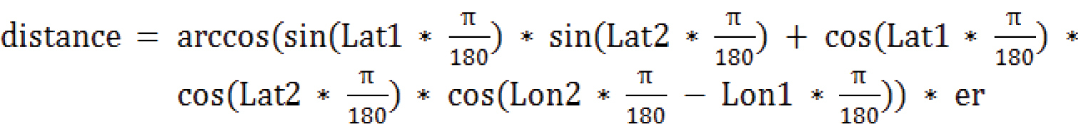
The earth’s radius (= er) in central Europe is 6,367 km. Lat1 and Lon1 are the latitude and longitude of the location of specimen 1, Lat2 and Lon2 those of specimen 2. For the full dataset see Suppl. material
Haplotype analysis
A haplotype analysis was conducted with DNASP (
In a second run the sequences were grouped again by considering only non-synonymous changes. In this second step all synonymous changes were discarded. For this an interim sequence set with only non-synonymous changes was created (DNASP / Generate / Polymorphic Data File / “only Non-synonymous”) and afterwards the Haplotype file was built. Because of the unequal sampling with a bias to the German fauna within the GBOL-project, no comparative population analysis was possible.
The previous first haplotype data file was used as a basis for a TCS Networks analysis (
Haplotype richness estimation
The potential number of haplotypes for the complete distribution area was estimated with ESTIMATES 9.1.0 (
Results
Phylogenetic relationship of G. marginata with similar species
The minimum interspecific distance of G. marginata to other Glomeris species ranges from 12.9–15.9 % (see Table
| Species | Min. p-distance to G. marginata |
|---|---|
| Glomeris connexa | 12.9 % |
| Glomeris maerens-group | 13.1 % |
| Glomeris klugii/undulata | 13.4 % |
| Glomeris apuana | 14.2 % |
| Glomeris intermedia | 14.8 % |
| Glomeris hexasticha | 14.9 % |
| Glomeris annulata | 15.9 % |


The specimens of the G. maerens species-group cluster together with a minimum interspecific distance (10.5 %) to the other species, but the G. maerens specimens fall into three clades with a maximum intraspecific distance of up to 9.1 % (see Figure
Intraspecific variation of G. marginata
All 97 specimens of G. marginata form a well-supported clade (bootstrap value 100 %, not shown in Figure
Geographical relationship of G. marginata specimens
The specimens from northern Germany and eastern France show the lowest genetic distance (≈ 1 %) to the rest of all samples. The specimens from western and southern France show the highest median distance (≈ 3–4 %) to those of other populations (see Table
The 10 specimens with smallest and greatest median p-distance to the rest of samples.
| p-Distance | ||||
| SpecimenID | BioRegion | Median | Max | Mean |
| G.mar.40 | DE.NDTO | 0.6 % | 3.5 % | 1.2 % |
| G.mar.17 | DE.MGSW | 0.9 % | 4.0 % | 1.3 % |
| G.mar.58 | FR.CON | 0.9 % | 3.8 % | 1.4 % |
| G.mar.59 | FR.CON | 0.9 % | 3.8 % | 1.4 % |
| G.mar.61 | FR.CON | 0.9 % | 3.8 % | 1.4 % |
| G.mar.95 | DE.MGSW | 0.9 % | 3.8 % | 1.4 % |
| G.mar.04 | DE.MGSO | 1.1 % | 3.8 % | 1.4 % |
| G.mar.05 | DE.MGSO | 1.1 % | 3.8 % | 1.4 % |
| G.mar.06 | DE.MGSO | 1.1 % | 3.8 % | 1.4 % |
| G.mar.07 | DE.MGSO | 1.1 % | 3.8 % | 1.4 % |
| … | … | … | … | … |
| G.mar.85 | FR.ATLN | 3.2 % | 4.9 % | 2.8 % |
| G.mar.86 | FR.ATLN | 3.2 % | 4.9 % | 2.8 % |
| G.mar.68 | FR.MED | 3.3 % | 4.7 % | 3.4 % |
| G.mar.65 | FR.MED | 3.5 % | 4.6 % | 3.4 % |
| G.mar.66 | FR.MED | 3.5 % | 4.6 % | 3.4 % |
| G.mar.67 | FR.MED | 3.5 % | 4.6 % | 3.4 % |
| G.mar.79 | FR.PYRN | 3.8 % | 4.9 % | 3.7 % |
| G.mar.77 | FR.PYRN | 3.8 % | 4.6 % | 3.8 % |
| G.mar.76 | FR.PYRN | 4.0 % | 5.0 % | 3.9 % |
| G.mar.71 | FR.MED | 4.0 % | 5.0 % | 3.9 % |
The maximum and the mean p-distance of G. marginata within the north-eastern part of the distribution (≈ 4 % or ≈ 1 %, respectively) is lower than in the south-western part (≈ 5 % or ≈ 3–4 %, respectively). Specimens from Mediterranean France group most distantly from the rest, with a maximum p-distance of 5.0 %.
The plot of the genetic p-distance to the geographical distances of all samples (4,656 possible pairs) shows no distinct relationship between both values (see Figure

Examples of specimen pairs with small and great ratio of p-distance (p-dist.) to geographical distance (geo-dist in km). Green marked: specimen pairs with exceptionally high p-dist. but low geo-dist. (representative for dots of upper-left side of Figure
| SpecimenID | SpecimenID | geo-dist | p-dist | p-dist./geo-dist. |
|---|---|---|---|---|
| G.mar.71 (FR.MED) | G.mar.79 (FR.PYRN) | 322 | 4.9 % | 0.000151 |
| G.mar.77 (FR.PYRN) | G.mar.78 (FR.PYRN) | 43 | 3.8 % | 0.000883 |
| G.mar.26 (DE.MGSW) | G.mar.93 (DE.MGSW) | 9 | 3.0 % | 0.003204 |
| G.mar.26 (DE.MGSW) | G.mar.36 (DE.MGSW) | 8 | 2.9 % | 0.003486 |
| G.mar.30 (DE.MGSW) | G.mar.31 (DE.MGSW) | 0 | 1,8 % | – |
| … | … | … | … | … |
| G.mar.57 (FR.ATLN) | G.mar.74 (FR.MED) | 647 | 0.2 % | 0.000002 |
| G.mar.01 (DE.MGSO) | G.mar.54 (FR.ALP) | 820 | 0.2 % | 0.000002 |
| G.mar.44 (DE.NDTO) | G.mar.84 (FR.ATLN) | 868 | 0.0 % | – |
| G.mar.43 (DE.NDTO) | G.mar.54 (FR.ALP) | 1031 | 0.0 % | – |
| G.mar.40 (DE.NDTO) | G.mar.52 (ES.PYRS) | 1610 | 0.6 % | 0.000004 |
Haplotypes/regions
Within the 657 sites of the 97 sequences of G. marginata, 74 were polymorphic which resulted from a total number of 81 mutations. The total number of synonymous changes is 71 and the total number of replacement changes is six. In the haplotype analysis, within the 97 samples, 47 haplotypes were detected, with 79 polymorphic sites. Haplotype diversity is 0.93, nucleotide diversity Pi is 0.017.
38 haplotypes (81 % of all haplotypes) consist of only one specimen (^ = 38 specimens ≙ 39 % of all specimens) and 42 haplotypes (89 % of all haplotypes) represents only specimens from one bioregion (^ = 48 specimens ^ = 49 % of all specimens). Nine haplotypes are represented in our dataset with two or more specimens (^ = 59 specimens ^ = 61 % of all specimens).
The dataset was divided into five major haplotype lineages (see Figure
Number of samples and bioregions (BioR) to major haplotypes (mHapT) and lineages.
| Number of lineages in Figure |
Number of Samples in mHapT | Number of BioR/mHapT BioR/lineage | Covered BioR | Number of Samples/lineages |
|---|---|---|---|---|
| I | 15 | 5 | DE.MGSW – DE.MGSO – DE.NDTO DE.SSL – FR.ALP | 17 |
| II | 17 | 4 | DE.MGSW – DE.MGSO – DE.NDTO FR.ATLN | 26 |
| III | 10 | 3/5 | DE.MGSW – FR.ATLN – GB.EM DE.NDTW – FR.CONS | 15 |
| IV | 4 | 2/3 | DE.MGSW – FR.CONN – DE.NDTW | 9 |


TCS-Network of haplotypes of Glomeris marginata with distribution region. Numbers behind region = consecutive haplotype number of DNASP-output. Haplotype accumulations: Red oval = Haplotype lineage I; Yellow oval = Haplotype lineage II; Blue oval = Haplotype lineage III; Green circle = Haplotype lineage IV; Black oval = Haplotype lineage V. Dashes on node connecting lines are representing single nucleotide mutations.
The other four haplotype lineages I–IV show a wider area of distribution, but genetically less diversity. Major haplotype lineages I and IV are closely related (see Figure
Haplotype lineage I occurs in an area reaching from the French Alps to NE Europe, with the main haplotype diversity in the German “Mittelgebirgsschwelle“, eastern part (DE.MGSO). Haplotype lineage II shows a central distribution with a high proportion of specimens in the German “Mittelgebirgsschwelle“, western part (DE.MGSW). Lineage II has the greatest distribution area and includes several subordinated haplotypes in the region DE.MGSW. Haplotype lineage III occurs in NW Europe with the most specimens in the France Atlantique, northern part (FR.ATLN). Additionally, the specimen from Great Britain (GB.EM) belongs to this group and has even the same haplotype as the majority specimens of this lineage. Haplotype lineage IV has a more narrow distribution range, with its main samples in France Continentale, northern part (FR.CONN). None of those four lineages are found in southern France or northern Spain (the distribution area of lineage V), but the distribution areas of the lineages I–IV overlap in DE.MGSW.
Haplotype lineages I–III and partially lineage IV are especially poor in haplotypes. Four haplotypes, one in each lineage (see Table
Every well-sampled bioregion has many haplotypes. The haplotype/specimen-rate is always higher than 0.3 (see Table
The haplotype lineage III mainly connects the northern French bioregion (FR.ATLN) with central Germany (DE.MGSW). One direct connection exists between the southern French/Spanish (FR.MED, FR.PYR and ES.CC) and the northern French populations (specimen 57, FR.ATLN, Table
Rates of haplotypes (HapT) and haplogroups (HapG) per samples in major sampled bioregions (BioR).
| BioRegion | Samples in BioR | HapT in BioR | HapT/Samples | Mean p-distance | HapG in BioR | HapG/Samples |
|---|---|---|---|---|---|---|
| Total | 97 | 47 | 0.5 | 1.9 % | 8 | 0.1 |
| DE.MGSW | 31 | 15 | 0.5 | 1.4 % | 4 | 0.1 |
| FR.ATLN | 14 | 7 | 0.5 | 1.9 % | 2 | 0.1 |
| DE.MGSO | 11 | 4 | 0.4 | 0.4 % | 2 | 0.2 |
| FR.MED | 11 | 8 | 0.7 | 2.2 % | 2 | 0.2 |
| DE.NDTO | 6 | 4 | 0.7 | 0.8 % | 1 | 0.2 |
| FR.CONN | 6 | 4 | 0.7 | 0.2 % | 1 | 0.2 |
| ES.CC | 4 | 4 | 1.0 | 0.6 % | 1 | 0.3 |
| FR.PYRN | 4 | 4 | 1.0 | 2.1 % | 2 | 0.5 |
| N-Europe | 77 | 30 | 0.4 | 1.8 % | 6 | 0.1 |
| S-Europe | 20 | 17 | 0.9 | 2.5 % | 3 | 0.2 |
Haplotype network of G. marginata
Based on the 47 haplotypes the TCS analysis shows a complex net of different possible evolutionary pathways between the haplotypes (see Figure
Haplotype number estimation
The rarefaction curve shows no saturation for the number of haplotypes (see Figure


Extrapolation of rarefaction curves with ESTIMATES of the COI sequences of Glomeris marginata. Blue line = estimation with premise of mean number (404 haplotypes); Horizontal yellow line = 95% satisfaction of mean number (384 haplotypes); Green and red line = curve at the 95% upper and lower boundary.
Colour morphs of G. marginata
The dataset contains one specimen of the grey colour morph, eight with the “perplexa” pattern and four with red margins. Those 13 distinctly coloured specimens are marked in our specimen tree (see Figure
Discussion
Glomeris annulata, G. apuana, and G. maerens
The three local endemic species, despite some similarities in the coloration (Figures
Further studies should investigate the G. maerens-group in northern Spain. All three species (G. maerens, G. lugubris Attems, 1927, and G. obsoleta Attems, 1952) of the group were described by Attems from Spain (G. maerens: Tarragona and Lérida; G. lugubris: Cádiz; G. obsoleta: Barcelona) and show a similar obscure black-brown colouration (see examples in Figure
Monophyly of G. marginata
Glomeris marginata is genetically distant but related to G. connexa, with a p-distance of 12.9 %. Based on the COI-data, the G. maerens species group is more closely related to G. connexa/G. apuana than to G. marginata. The genetic distance of G. marginata to the other tested species (G. klugii/undulata, G. intermedia, G. hexasticha, and G. annulata) is, with a p-distance up to 15.9 %, even more pronounced.
In comparison to vertebrate species (e.g., fishes: 0.32 %,
The known colour morphs of G. marginata do not represent single lineages or even subspecies. The conspicuously red borders in specimens from southern France (Figures
The COI-gene is clearly working as a barcoding gene to identify and discriminate G. marginata specimens from the other Glomeris species.
Geographical relationship of G. marginata specimens
Syntopical specimens as well as specimens with a maximum geographical distance of 1,701 km (Germany, Brandenburg to Spain, La Rioja) were analysed. There is no obvious relationship between geographical and genetic distance. There are specimen pairs of the same haplotype (p-distance = 0) which were collected more than 1,000 km apart. This distance of 1,000 km seems to be the maximum distance G. marginata could spread without experiencing genetic changes. Specimen pairs with a geographical distance larger than 1,000 km experienced at least a few mutations in the COI gene, with a minimum p-distance of ≈ 0.8 % in our dataset (see Figure
On the other hand, local specimens can show high genetic variation. Even from nearby locations specimen pairs show a p-distance as high as 3 %. Such a mutation rate is unlikely to have happened locally, but is more likely the result of a different geographical origin of the source populations. As such large genetic distances between different populations of G. marginata are common, a human-influenced dispersal seems not to be the reason behind the regular high COI-variance.
Haplotype regions, origin and potential migration patterns
The haplotype analysis shows five main haplotype lineages in G. marginata (Figure
The haplotype lineage V is highly genetically variable, therefore a combination into a single group is not justified. Four rather distinct lineages not forming a monophylum could be seen in Figure
The examined northern European regions are mainly inhabited by specimens of the haplotype lineages I–IV, showing a low variance in their p-distance to one another (see Table
With the before mentioned mean p-distance of 2.5 %, the small south European area of bioregions contains a much higher genetic diversity in G. marginata than the much larger northern Europe. To develop such a higher genetic diversity, the south European populations of G. marginata must be older than the northern European populations. Northern Europe must have been colonized by G. marginata more recently. The main dispersal into those northern areas could only have been started after the last glaciation retreated during the early Holocene starting around 11,000 years ago (
Our data does not reveal how far north the distribution of G. marginata reached and how high any genetic diversity of the species was before the ice age. However, the south European mixed populations could be regarded as a remnant of old haplotype lineages of G. marginata, which are not any more present in the north European populations.
The geographical coverage of our analysed specimens is biased towards western Germany (MGSW, see Figure
Contrarily, all main haplotype lineages I–IV, which are exclusively found in northern Europe are linked to the bioregion DE.MGSW (Figure
Haplotype number estimation
With this work, for the first time, a survey of almost 100 barcodes is presented for a diplopod species. On average, every haplotype in our study is based on two specimens (97 specimens / 47 haplotypes). In reality, the majority of haplotypes (38 haplotypes ^ = 81 %) are represented by only one specimen. The haplotype number estimation has shown that these 97 successfully sequenced specimens are just providing an overview of the real haplotype diversity in G. marginata. With the current data we are still far away from a complete collection of all haplotypes of the species. Many more specimens need to be collected to reach at least the lower estimated boundary of 140 haplotypes.
In general, this also means that haplotype analysis should not be based on few specimens and not only on specimens of a certain region, but always from specimens covering the whole distribution area of a species (
Many new haplotypes would simply represent the missing mutation steps present in the TCS-network of Figure
Nomenclatorial acts
In the year 1789 the species with the common name Cloporte bordé (bordered woodlouse) was first described by the French naturalist Charles Joseph de Villers (1724–1810) as Oniscus marginatus. He used few, but descriptive words: “niger, segmentis corporis luteo marginatis” [black, segments of the body with yellow margin].
Within a few years the species has been named and described four times again (see below). Thirteen years after the description the French zoologist Pierre André Latreille (1762–1833) placed the species in his new genus Glomeris Latreille, 1802. Almost one hundred years later several subspecies or variations were added by Verhoeff, Latzel, and Attems. Those taxa represent different versions of the pale form which was first named G. perplexa by
We do not recognize any subspecies of G. marginata. Therefore the subspecies Glomeris marginata ponentina Verhoeff, 1911 and Glomeris marginata leridana Attems, 1927 are synonymised under the nominal species.
Only initial new naming acts are listed. Due to the numerous mentions of G. marginata in the literature, a comprehensive list of all citations is not provided.
Glomeris marginata (Villers, 1789)
Oniscus marginatus Villers, 1789: 187 (first description, type locality “Gallia australiori” – south France)
Glomeris marginata – Latreille, 1802: 66 (placing the taxon in the genus Glomeris)
Synonyms
Julus limbatus Olivier, 1792: 414 = Glomeris limbatus (Latreille, 1802: 66)
Armadillo marginalis Culver, 1792: 30, fig. 23–25, new synonym
Oniscus zonatus Panzer, 1793: Heft 9, chapter 25
Julus oniscoides Steward, 1802, chapter V: 307
Glomeris marginata var. lucida Latzel, 1890: 365 and 367
Glomeris perplexa Latzel, 1895: 7 and 11, new synonym
Glomeris connexa perplexa Verhoeff, 1906: 152
Glomeris connexa perplexa aberr. rhenanorum Verhoeff, 1906: 152 and 153
Glomeris connexa perplexa var. rhenana Verhoeff, 1906: 152
Glomeris marginata aut. genuina Verhoeff, 1911: 121
Glomeris marginata var. marginata Verhoeff, 1911: 121
Glomeris marginata var. perplexa Verhoeff, 1911: 121
Glomeris marginata ponentina Verhoeff, 1911: 122, new synonym
Glomeris marginata leridana Attems, 1927: 250, new synonym
The description of Oniscus variegatus Villers, 1789: 188, fig. 16 (“niger, segmentis corporis nigris, albo marginatis …” - black, the segments of the body black, white framed) also perfectly fits G. marginata and therefore could potentially be treated as a junior synonym of it. However, with the case 2909 of the International Commission on Zoological Nomenclature it was already treated as a senior synonym of Armadillidium vulgare Latreille, 1804 and placed on the Official Index of Rejected and Invalid Species Names in Zoology (
Analysis software used in this study
BIOEDIT 7.2.5: http://www.mbio.ncsu.edu/bioedit/bioedit.html
DNASP 5.10.1: http://www.ub.edu/dnasp
ESTIMATES 9.1.0: http://viceroy.eeb.uconn.edu/estimates
FIGTREE 1.4.2: http://tree.bio.ed.ac.uk/software/figtree
GLOBALMAPPER 17: http://www.bluemarblegeo.com/products/global-mapper.php
MEGA 7.14 GUI: http://www.megasoftware.net
MICROSOFT EXCEL 2013: http://www.microsoftstore.com
POPART 1.7: http://popart.otago.ac.nz
Acknowledgements
B. Rulik, J. Thormann, and L. von der Mark from the GBOL-Team in Bonn who photographed, extracted and sequenced the G. marginata ZFMK specimens; their invaluable help is greatly appreciated. M. Geiger assisted with the upload of the sequence data to GenBank. Specimens of the outgroup taxa were thankfully prepared and sequenced by Claudia Etzbauer (ZFMK). Specimens were thankfully provided by Peter Kautt, Axel Schönhofer, Helen Read, and Robin Duborget. We thank Michaël Aubert of the University of Rouen for providing us the sequences and data of specimens from France, Haut Normandie (via BOLD).
We also thank Jörg Spelda (Munich) and Hans Pohl (Jena) for discussions on the earlier version of the manuscript, Henrik Enghoff (Copenhagen) and an anonymous reviewer provided numerous comments that greatly enhanced the quality of the here presented work. We are indebted to Steve Gregory (Oxford) for improving our English. This is a publication of the German Barcode of Life (GBOL) project of the Humboldt Ring, financed by the German Federal Ministry for Education and Research (FKZ 01LI1101A and FKZ 01LI1101B).
References
- Aho K, Derryberry D, Peterson T (2014) Model selection for ecologists: the worldviews of AIC and BIC. Ecology 95: 631–636. https://doi.org/10.1890/13-1452.1
- Ansenne A, Compère P, Goffinet G (1990) Ultrastructural organization and chemical composition of the mineralized cuticle of Glomeris marginata (Myriapoda, Diplopoda). In Minelli A (Ed.) Proceedings of the 7th International Congress of Myriapodology. Brill, Leiden, 125–134.
- Attems C (1927) Myriopoden aus den nördlichen und östlichen Spanien, gesammelt von Dr. F. Haas in den Jahren 1914–1919. Nebst Beiträgen zur Kenntnis der Lithobiiden, Glomeriden sowie der Gattungen Brachydesmus und Archiulus. Abhandlungen der Senckenbergischen naturforschenden Gesellschaft 39(3): 233–289.
- Attems C (1952) Myriopoden der Forschungsreise Dr. H. Franz in Spanien 1951 nebst Übersicht über die gesamte iberische Myriopodenfauna. EOS, Revista Espanola de Entomologia 28(4): 323–366.
- Bergsten J, Bilton DT, Fujisawa T et al. (2012) The effect of geographical scale of sampling on DNA barcoding. Systematic Biology 61: 851–869. https://doi.org/10.1093/sysbio/sys037
- Candia Carnevali MD, Valvassori R (1982) Active supercontraction in rolling-up muscles of Glomeris marginata (Myriapoda, Diplopoda). Journal of Morphology 172(1): 75–82. https://doi.org/10.1002/jmor.1051720107
- Carrel JE (1984) Defensive secretion of the pill millipede Glomeric [Glomeris] marginata. 1. Fluid production and storage. Journal of Chemical Ecology 10(1): 41–51. https://doi.org/10.1007/BF00987642
- Chao A (1984) Nonparametric Estimation of the Number of Classes in a Population. Scandinavian Journal of Statistics 11(4): 265–270.
- Clement M, Snell Q, Walker P, Posada D, Crandall K (2002) TCS: Estimating gene genealogies. Parallel and Distributed Processing Symposium, International Proceedings 2: 184. https://doi.org/10.1109/IPDPS.2002.1016585
- Colwell RK (2013) EstimateS: Statistical estimation of species richness and shared species from samples. Version 9. http://purl.oclc.org/estimates
- Colwell RK, Chao A, Gotelli NJ, Lin SY, Mao CX, Chazdon RL, Longino JT (2012) Models and estimators linking individual-based and sample-based rarefaction, extrapolation, and comparison of assemblages. Journal of Plant Ecology 5: 3–21. https://doi.org/10.1093/jpe/rtr044
- Compère PS, Defise S, Goffinet G (1996) Cytochemistry of the tergite epicuticle of Glomeris marginata (Villers) (Myriapoda, Diplopoda): preliminary experimental results. Mémoires du Muséum national d’Histoire naturelle 169: 395–401.
- Cuvier G (1792) Mémoire sur les cloportes terrestres. Journal d’Histoire naturelle (Paris) 2(13): 18–31.
- David JF, Gillon D (2002) Annual feeding rate of the millipede Glomeris marginata on holm oak (Quercus ilex) leaf litter under Mediterranean conditions. Pedobiologia 46(1): 42–52. https://doi.org/10.1078/0031-4056-00112
- Dohle W (1964) Die Embryonalentwicklung von Glomeris marginata (Villers) im Vergleich zur Entwicklung anderer Diplopoden. Zoologische Jahrbücher / Abteilung für Anatomie und Ontogenie der Tiere 81: 241–310.
- Dove H, Stollewerk A (2003) Comparative analysis of neurogenesis in the myriapod Glomeris marginata (Diplopoda) suggests more similarities to chelicerates than to insects. Development 130: 2161–2171. https://doi.org/10.1242/dev.00442
- Dunger W, Steinmetzger K (1981) Ökologische Untersuchungen an Diplopoden einer Rasen-Wald-Catena im Thüringer Kalkgebiet. Zoologische Jahrbücher, Abteilung für Systematik, Ökologie und Geographie der Tiere 108(4): 519–553.
- Elias M, Hill RI, Willmott KR et al. (2007) Limited performance of DNA barcoding in a diverse community of tropical butterflies. Proceedings of the Royal Society B: Biological Sciences 274: 2881–2889. https://doi.org/10.1098/rspb.2007.1035
- Enghoff H, Dohle W, Blower JG (1993) Anamorphosis in millipedes (Diplopoda) - the present state of knowledge with some developmental and phylogenetic considerations. Zoological Journal of the Linnean Society 109: 103–234. https://doi.org/10.1111/j.1096-3642.1993.tb00305.x
- Fusco G, Minelli A (2013) Arthropod Segmentation and Tagmosis. In: Minelli A (Ed.) Arthropod Biology and Evolution, 91–122. https://doi.org/10.1007/978-3-662-45798-6_9
- Gotelli NJ, Colwell RK (2010) Estimating species richness. In: Biological Diversity: Frontiers In: Magurran AE, McGill BJ (Eds) Measurement and Assessment. Oxford University Press, Oxford, 39–54.
- Haacker U (1964) Das Paarungsverhalten des Saftkuglers Glomeris marginata. Natur und Museum 94: 265–272.
- Hall TA (1999) BioEdit: a user-friendly biological sequence alignment editor and analysis program for Windows 95/98/NT. Nucleic Acids Symposium Series 41: 95–98.
- Hilken G (1998) Vergleich von Tracheensystemen unter phylogenetischem Aspekt. Verhandlungen des naturwissenschaftlichen Vereins Hamburg (N.F. ) 37: 5–94.
- Hilken G, Sombke A, Müller CHG, Rosenberg J (2015) Diplopoda - tracheal system. In: Minelli A (Ed.) Treatise on zoology - anatomy, taxonomy, biology. The Myriapoda 2(6), 129–152. https://doi.org/10.1163/9789004188273_007
- Hoess R (2000) Bestimmungsschlüssel für die Glomeris-Arten Mitteleuropas und angrenzender Gebiete (Diplopoda: Glomeridae). Jahrbuch des Naturhistorischen Museums Bern 13: 3–20.
- International Commission on Zoological Nomenclature (1998) Glomeris Latreille, 1802 (Diplopoda), Armadillo Latreille, 1802, Armadillidium Brandt in Brandt and Ratzeburg, (1831) and Armadillo vulgaris Latreille, 1804 (currently Armadillidium vulgare) (Crustacea, Isopoda): Generic and specific names conserved. Bulletin of Zoological Nomenclature 55(2): 124–12.
- Janssen R (2004) Untersuchungen zur molekularen Grundlage der Segmentbildung im Saftkugler Glomeris marginata (Myriapoda: Diplopoda). Inaugural-Dissertation zur Erlangung des Doktorgrades an der Mathematisch-Naturwissenschaftlichen Fakultät der Universität zu Köln, 313 pp.
- Janssen R, Prpic NM, Damen WGM (2006) Dorso-ventral differences in gene expression in Glomeris marginata (Villers, 1789) (Myriapoda: Diplopoda). Norwegian Journal of Entomology 53(2): 129–137.
- Janssen R, Damen WGM (2006) The ten Hox genes of the millipede Glomeris marginata. Development, Genes and Evolution 216(7–8): 451–465. https://doi.org/10.1007/s00427-006-0092-5
- Janssen R (2011) An abnormally developed embryo of the pill millipede Glomeris marginata that lacks dorsal segmental derivatives. Development, Genes and Evolution 221: 351–355. https://doi.org/10.1007/s00427-011-0377-1
- Janssen R (2013) Developmental abnormalities in Glomeris marginata (Villers 1789) (Myriapoda: Diplopoda): implications for body axis determination in a myriapod. Naturwissenschaften 100: 33–43. https://doi.org/10.1007/s00114-012-0989-y
- Janssen R, Posnien N (2014) Identification and embryonic expression of Wnt2, Wnt4, Wnt5 and Wnt9 in the millipede Glomeris marginata (Myriapoda: Diplopoda). Gene Expression Patterns 14: 55–61. https://doi.org/10.1016/j.gep.2013.12.003
- Johnson IT, Riegel JA (1977a) Ultrastructural studies on the Malpighian tubule of the pill millipede, Glomeris marginata (Villers). Cell and Tissue Research 180(3): 357–366. https://doi.org/10.1007/BF00227601
- Johnson IT, Riegel JA (1977b) Ultrastructural tracer studies on the permeability of the Malpighian tubule of the pill millipede, Glomeris marginate (Villers). Cell and Tissue Research 182(4): 549–56. https://doi.org/10.1007/BF00219837
- Jordan HB, Kambestadt M (2014) DNA barcoding of bark and ambrosia beetles reveals excessive NUMTs and consistent east-west divergence across Palearctic forests. Molecular Ecology Resources 14: 7–17. https://doi.org/10.1111/1755-0998.12150
- Juberthie-Jupeau L (1967) Les oothèques de quelques Diplopodes Glomeridia. Revue d'Ecologie et de Biologie du Sol 4: 131–142.
- Juberthie-Jupeau L (1978) Fine structure of postgonopodial glands of a myriapod Glomeris marginata (Villers). Tissue and Cell 8(2): 293–304. https://doi.org/10.1016/0040-8166(76)90053-7
- Lehtinen PT, Holthuis LB (1995) Glomeris Latreille, 1802 (Diplopoda): Proposed conservation; Armadillo vulgaris Latreille, 1804 (Crustacea, Isopoda): Proposed conservation of the specific name; and Armadillo Latreille, 1802 (Crustacea, Isopoda): Application for a ruling on its status. Bulletin of Zoological Nomenclature 52(3): 236–243. https://doi.org/10.5962/bhl.part.6782
- Librado P, Rozas J (2009) DnaSP v5: A software for comprehensive analysis of DNA polymorphism data. Bioinformatics 25: 1451–1452. https://doi.org/10.1093/bioinformatics/btp187
- Keskin E, Atar HH (2013) DNA barcoding commercially important fish species of Turkey. Molecular Ecology Resources 13: 788–797. https://doi.org/10.1111/1755-0998.12120
- Kime RD, Enghoff H (2011) Atlas of European Millipedes (Class Diplopoda), Vol. 1 - Orders Polyxenida, Glomerida, Platydesmida, Siphonocryptida, Polyzoniida, Callipodida, Polydesmida. Series: Fauna Europeaea Evertebrata #3, Pensoft Publishers, 282 pp.
- Koch M (2015) Diplopoda - general morphology. In: Minelli A (Ed.) Treatise on zoology - anatomy, taxonomy, biology. The Myriapoda 2(2), 7–68. https://doi.org/10.1163/9789004188273_003
- Kumar S, Stecher G, Tamura K (2015) MEGA7: Molecular Evolutionary Genetics Analysis version 7.0 for bigger datasets. Molecular Biology and Evolution 33(7): 1870–1874. https://doi.org/10.1093/molbev/msw054
- Latzel R (1890) Description d’une variété nouvelle du Glomeris marginata Villers. In: Gadeau de Kerville H (1890) Deuxième addenda à la faune des myriopodes de la Normandie. Bulletin de la Société des Amis des Sciences naturelles de Rouen 1889(1): 363–367.
- Latzel R (1895) Die Myriopoden aus der Umgebung Hamburgs. Jahrbuch der Hamburgischen Wissenschaftlichen Anstalten, Beiheft 12: 99–109.
- Latreille PA (1802) Histoire naturelle, générale et particulière des Crustacés et des Insectes. 3 + 7. (= Tom 95 + 99), Dufart, Paris, 467 pp.
- Li J, Zheng X, Cai Y, Zhang X, Yang M, Yue B, Li J (2015) DNA barcoding of Murinae (Rodentia: Muridae) and Arvicolinae (Rodentia: Cricetidae) distributed in China. Molecular Ecology Resources 15: 153–167. https://doi.org/10.1111/1755-0998.12279
- Martin JS, Kirkham JB (1989) Dynamic role of microvilli in peritrophic membrane formation. Tissue and Cell 21: 627–638. https://doi.org/10.1016/0040-8166(89)90013-X
- Meynen E, Schmithüsen J (1953–1962) Handbuch der naturräumlichen Gliederung Deutschlands. Bundesanstalt für Landeskunde, Remagen/Bad Godesberg. 9 issues in 8 books, actualized map 1:1.000.000 (1960).
- Meinwald YC, Meinwald J, Eisner T (1966) 1,2-Dialkyl-4 (3H)-quinqzolinones in the defensive secretion of a millipede (Glomeris marginata). Science (Washington DC) 154(3747): 390–391. https://doi.org/10.1126/science.154.3747.390
- Minelli A, Fusco G (2013) Arthropod Post-embryonic Development. In: Minelli (Ed) Arthropod Biology and Evolution, 91–122. https://doi.org/10.1007/978-3-662-45798-6_5
- Minelli A (2015) Diplopoda - development. In: Minelli A (Ed.) Treatise on zoology - anatomy, taxonomy, biology. The Myriapoda 2(1), 267–302. https://doi.org/10.1163/9789004188273_012
- Müller CHG, Sombke A (2015) Diplopoda - sense organs. In: Minelli A (Ed.) Treatise on zoology - anatomy, taxonomy, biology. The Myriapoda 2(9), 181–236.
- Nicholson PB, Bocock KL, Heal OW (1966) Studies on the decomposition of the faecal pellets of a millipede [Glomeris marginata (Villers)]. Journal of Ecology 54: 755–766. https://doi.org/10.2307/2257815
- Olivier AG (1792) Encyclopédie méthodique. Dictionnaire des Insectes, vol. 7. Paris, 827 pp.
- Panzer W (1793–1813) Faunae Insectorum Germaniae initia. Nürnberg, Vol. 2, issue 9.
- Prpic NM, Tautz D (2003) The expression of the proximodistal axis patterning genes Distal-less and dachshund in the appendages of Glomeris marginata (Myriapoda: Diplopoda) suggests a special role of these genes in patterning the head appendages. Developmental Biology 260: 97–112. https://doi.org/10.1016/S0012-1606(03)00217-3
- Prpic NM (2004) Homologs of wingless and decapentaplegic display a complex and dynamic expression profile during appendage development in the millipede Glomeris marginata (Myriapoda: Diplopoda). Frontiers in Zoology 1(6): 1–12.
- Prpic NM (2005) Duplicated Pax6 genes in Glomeris marginata (Myriapoda: Diplopoda), an arthropod with simple lateral eyes. Zoology (Jena) 108(1): 47–53. https://doi.org/10.1016/j.zool.2004.11.003
- Prpic NM, Janssen R, Damen WGM, Tautz D (2005) Evolution of dorsal-ventral axis formation in arthropod appendages: H15 and optomotor-blind/bifid-type T-box genes in the millipede Glomeris marginata (Myriapoda: Diplopoda). Evolution and Development 7(1): 51–57. https://doi.org/10.1111/j.1525-142X.2005.05006.x
- Rawlins AJ, Bull ID, Poirier N, Ineson P, Evershed RP (2006) The biochemical transformation of oak (Quercus robur) leaf litter consumed by the pill millipede (Glomeris marginata). Soil Biology & Biochemistry 38: 1063–1076. https://doi.org/10.1016/j.soilbio.2005.09.005
- Regier JC, Shultz JW (2001) A phylogenetic analysis of Myriapoda (Arthropoda) using two nuclear protein-encoding genes. Zoological Journal of the Linnean Society 132(4): 469–486. https://doi.org/10.1111/j.1096-3642.2001.tb02471.x
- Regier JC, Wilson HM, Shultz JW (2005) Phylogenetic analysis of Myriapoda using three nuclear protein-coding genes. Molecular phylogenetics and evolution 34(1): 147–158. https://doi.org/10.1016/j.ympev.2004.09.005
- Reip HS, Spelda J, Voigtländer K, Decker P, Lindner EN (2016) Rote Liste und Gesamtartenliste der Doppelfüßer (Myriapoda: Diplopoda) Deutschlands. In: Gruttke H, Binot-Hafke M, Balzer S, Haupt H, Hofbauer N, Ludwig G, Matzke-Hajek G, Ries M (Eds) Rote Liste gefährdeter Tiere, Pflanzen und Pilze Deutschlands, Band 4: Wirbellose Tiere (Teil 2). Landwirtschaftsverlag, Münster. Naturschutz und Biologische Vielfalt 70(4), 301–324.
- Roberts N (2014) The Holocene: An Environmental History, Wiley-Blackwell, Hoboken, 376 pp.
- Sahli F (1966) Contribution à l'étude de la périodomorphose et du système neurosécréteur des Diplopodes Iulides. Thèse Doctoral Sciences, Université de Bourgogne, Dijon 94, 226 pp.
- Seifert G (1966) Das stomatogastriche Nervensystem der Diplopoden. Zoologische Jahrbücher / Abteilung für Anatomie und Ontogenie der Tiere 83: 449–492.
- Schildknecht H, Wenneis WF, Weis KH, Maschwitz U (1966) Glomerin, ein neues Arthropoden-Alkaloid. Zeitschrift für Naturforschung 21 B(2): 121–127. https://doi.org/10.1515/znb-1966-0206
- Schildknecht H, Maschwitz U, Wenneis WF (1967) Über Arthropoden-Abwehrstoffe XXIV. Neue Stoffe aus dem Wehrsekret der Diplopodengattung Glomeris. Naturwissenschaften 54: 196–197. https://doi.org/10.1007/BF00594514
- Schildknecht H, Wenneis WF (1967) Über Arthropoden-Abwehrstoffe XX. Strukturaufklärung des Glomerins. Zeitschrift für Naturforschung C 21: 552–556.
- Schlüter U (1980) Die Feinstruktur der Pylorusdrüsen von Polydesmus angustus Latzel und Glomeris marginata Villers (Diplopoda). Zoomorphology 94: 307–319. https://doi.org/10.1007/BF00998207
- Schubart O (1934) Tausendfüßler oder Myriapoda. I: Diplopoda. In: Dahl F (Ed. ) Die Tierwelt Deutschlands und der angrenzenden Meeresteile, vol. 28, 318 pp.
- Spelda J, Reip HS, Oliveira-Biener U, Melzer RR (2011) Barcoding Fauna Bavarica: Myriapoda - a contribution to DNA sequence-based identifications of centipedes and millipedes (Chilopoda, Diplopoda). ZooKeys 156: 123–139. https://doi.org/10.3897/zookeys.156.2176
- Charles S (1802) Elements of Natural History. Volume II, London, 491 pp.
- Tamura K, Stecher G, Peterson D, Filipski A, Kumar S (2013) MEGA6: Molecular Evolutionary Genetics Analysis Version 6.0. Molecular Biology and Evolution 30: 2725–2729. https://doi.org/10.1093/molbev/mst197
- Tavaré S (1986) Some Probabilistic and Statistical Problems in the Analysis of DNA Sequences. Lectures on Mathematics in the Life Sciences (American Mathematical Society) 17: 57–86.
- Van der Drift J (1975) The significance of the millipede Glomeris marginata (Villers) for oaklitter decomposition and an approach of its part in energy flow. In: Vanek J (Ed.) Progress in soil zoology. Junk, The Hague, 293–298. https://doi.org/10.1007/978-94-010-1933-0_32
- Verhoeff KW (1895) Ein Beitrag zur Kenntnis der Glomeriden. Verhandlungen des naturhistorischen Vereins der Preußischen Rheinlande, Westfalens und des Regierungsbezirks Osnabrück 52: 221–234.
- Verhoeff KW (1906) Über Diplopoden. 4. (24.) Aufsatz: Zur Kenntnis der Glomeriden (zugleich Vorläufer einer Glomeris-Monographie) (Beiträge zur Systematik, Geographie, Entwickelung, vergleichenden Morphologie und Biologie). Archiv für Naturgeschichte 72(1): 107–226.
- Verhoeff KW (1911) Ueber Diplopoden. 20. (40.) Aufsatz: Neuer Beitrag zur Kenntnis der Gattung Glomeris. Jahreshefte des Vereins für vaterländische Naturkunde in Württemberg 67: 78–147.
- Villers CJ de (1789) Caroli Linnaei Entomologia, faunae Suecicae descriptionibus aucta Scopoli, Geoffroy, de Geer, Fabricii, Schrank. Volume 4, Aptera. Lugduni, 556 pp.
- Voigtländer K (2011) Preferences of common Central European millipedes for different biotope types (Myriapoda, Diplopoda) in Saxony-Anhalt (Germany). International Journal of Myriapodology 6: 61–83. https://doi.org/10.3897/ijm.6.2172
- Voigtländer K, Reip HS, Decker P, Spelda J (2011) Critical reflections on German Red Lists of endangered myriapod species (Chilopoda, Diplopoda) (with species list for Germany). International Journal of Myriapodology 6: 85–105. https://doi.org/10.3897/ijm.6.2175
- Vrieze SI (2012) Model selection and psychological theory: A discussion of the differences between the Akaike information criterion (AIC) and the Bayesian information criterion (BIC). Psychological Methods 17(2): 228–243. https://doi.org/10.1037/a0027127
- Wernitzsch W (1910) Beiträge zur Kenntnis von Craspedosoma simile und des Tracheensystems der Diplopoden. Jenaische Zeitschrift für Naturwissenschaft 39: 225–228.
- Wesener T (2015a) No millipede endemics north of the Alps? DNA-Barcoding reveals Glomeris malmivaga Verhoeff, 1912 as a synonym of G. ornata Koch, 1847 (Diplopoda, Glomerida, Glomeridae). Zootaxa 3999(4): 571–580. https://doi.org/10.11646/zootaxa.3999.4.7
- Wesener T (2015b) Integrative redescription of a forgotten Italian pill millipede endemic to the Apuan Alps - Glomeris apuana Verhoeff, 1911 (Diplopoda, Glomerida, Glomeridae). Zootaxa 4039(2): 391–400. https://doi.org/10.11646/zootaxa.4039.2.11
- Wesener T, Conrad C (2016) Local Hotspots of Endemism or Artifacts of Incorrect Taxonomy? The Status of Microendemic Pill Millipede Species of the Genus Glomeris in Northern Italy (Diplopoda, Glomerida). PLoS ONE 11(9): 1–22, e0162284. https://doi.org/10.1371/journal.pone.0162284
- Wesener T, Raupach MJ, Sierwald P (2010) The origins of the giant pill-millipedes from Madagascar (Diplopoda: Sphaerotheriida: Arthrosphaeridae). Molecular phylogenetics and evolution 57(3): 1184–1193. https://doi.org/10.1016/j.ympev.2010.08.023
- Wesener T, Voigtländer K, Decker P, Oeyen JP, Spelda J (2015) Barcoding of Central European Cryptops centipedes reveals large interspecific distances with ghost lineages and new species records from Germany and Austria (Chilopoda, Scolopendromorpha). ZooKeys 564: 21–46. https://doi.org/10.3897/zookeys.564.7535
Supplementary materials
Complete sequences dataset
Data type: FASTA format.
Explanation note: Complete sequences dataset of all specimens of this study in format FASTA.
P-distance matrix
Data type: Microsoft Excel Worksheet (.xls).
Explanation note: P-distance matrix over all specimens as EXCEL-file. Export from MEGA7.
P-distance – geographical distance
Data type: Microsoft Excel Worksheet (.xls).
Explanation note: P-distance – geographical distance table of all G. marginata specimens as EXCEL-file.
POPART-data
Data type: NEXUS format.
Explanation note: POPART-data file of haplotypes in format NEXUS.
ESTIMATES-data
Data type: Text Document (.txt).
Explanation note: ESTIMATES-data file of haplotypes as text file.