


(C) 2011 Sashi Bhushan Rao. This is an open access article distributed under the terms of the Creative Commons Attribution License, which permits unrestricted use, distribution, and reproduction in any medium, provided the original author and source are credited.
For reference, use of the paginated PDF or printed version of this article is recommended.
The cyst nematode Heterodera cajani is one of the major endemic diseases of pigeonpea, an important legume for food security and protein nutrition in India. It occurs in several pulse crops grown over a range of Indian agro climatic conditions but the extent of its intraspecific variation is inadequately defined. In view of this, 11 populations of Heterodera cajani were analyzed using morphometrics and the results correlated with those obtained from an AFLP approach using 24 primer pair combinations that amplified a total of 1278 AFLP markers. The cluster solution from this binary data indicated similarities for five populations that differed from those suggested by morphometrics. The differences obtained could not be related to geographic distance between populations. The data suggests that recent and long distance dispersal has occurred whose causes need to be defined to restrict further field introductions. Four AFLP primer pairs clustered the populations similarly to that generated using all 24 primer pairs. This simplified approach may provide a rapid basis for discriminating populations for their future management and help to check further distribution in agricultural trade. It may also have potential to determine differences in populations that relate to host range or virulence to resistance genes.
Heterodera cajani, pigeonpea cyst nematode, intraspecific variation, morphometrics, AFLP
The legume pigeonpea, (Cajanus cajan [L.] Millsp)is one of the most important pulse crops grown in India which produces 90% of the global production with over 100 cultivars on 2.4 million hectares. Outputs of over 750 Kg/ha about 50 years ago have now declined to 647kg/ha (www.icrisat.org). Diseases (Fusarium wilts, sterility mosaic) and pests such as pod borer and nematodes are all assumed to have contributed to the loss of productivity per hectare (www.icrisat.org). Heterodera cajani Koshy is the most important nematode pathogen of pigeonpea in India (
Knowledge of variability of an economic plant parasitic nematode species is important for the selection of appropriate control strategies (
AFLP is a useful approach for the genetic analysis of nematodes (
We have compared standard morphometric measurements for both J2 and the vulval cones of cysts with AFLP analysis for 11 populations of Heterodera cajani recovered from across India to determine the comparative utility of the three approaches to discriminate the populations. Cluster analysis was used to compare the relationships defined by the methods used. As a result, we report an AFLP-based approach for identifying major sub groups of Heterodera cajani in India. The results suggest that the current wide distribution of the populations in India is recent.
Material and methods Collection and multiplication of Heterodera cajani populationsSoil samples of 11 Heterodera cajani populations were collected during surveys, where pigeonpea is cultivated (Table 1). Populations were multiplied on pigeonpea plants growing in pots under glass house conditions to provide continuous stocks of encysted eggs for the work programme. Seventy-five days after adding cysts to plantlets, the soil in the culture pots was processed using Cobb’s sieving technique. Cysts were handpicked using a stereo binocular microscope and then processed for detailed morphological and genetic studies. Second stage juveniles (J2s) were expressed from their eggshells after opening cysts with needles.
Different Heterodera cajani populations collected from various agroclimatic regions of India
| Population Number | State | Locality |
|---|---|---|
| 1 | Uttar Pradesh | Allahabad |
| 2 | Andhra Pradesh | Hyderabad |
| 3 | Uttar Pradesh | Bahadurgarh |
| 4 | Uttar Pradesh | Kanpur 1 |
| 5 | Karnataka | Gulberga |
| 6 | Uttar Pradesh | Ghaziabad |
| 7 | Haryana | Hisar |
| 8 | Uttar Pradesh | Kanpur 2 |
| 9 | Delhi | Delhi |
| 10 | Tamil Nadu | Coimbatore |
| 11 | Uttar Pradesh | Meja |
The cyst vulval cones and J2 of populations were studied using light microscopy. The J2s were heat killed, fixed in 2% formaldehyde and processed following the method of
Genomic DNA was isolated by using Ultra pure Mammalian Genomic DNA Prep Kit (Bangalore Genei Pvt Ltd, Bangalore, India, Cat # KT-81). The quality and yield of genomic DNA was determined by running samples on 1% agarose gel. DNA concentrations were estimated spectrophotometrically (Perkin Elmer, Lambda-32, UV/visible, USA).
AFLP-PCRAFLP analysis was performed according to
PCR conditions were as follows: the preamplification mixture was prepared in a total volume of 50 µl and amplified using 20 cycles of 94°C for 30 s, 56°C for 30 s, and 72°C for 60 s. The following touchdown protocol was used for selective amplification in a 10-µl volume: 13 cycles of 94°C for 30 s, 65°C for 30 s with a decrease of –0.7°C per cycle, and 72°C for 1 min; followed by 23 cycles at the annealing temperature of 56°C. The PCR products from each primer combination were separated in 6% denaturing polyacrylamide gels in 1× TBE buffer and visualized with autoradiogram. AFLP bands were scored for absence (0) or presence (1) across the analyzed accessions for each primer combination.
Statistical approachesOne-way analysis of variance of variables for cyst cones and J2s were carried out usingSPSS version 16.0 with a priori contrasts between the reference population (Delhi) and each of the other populations. Cluster and related analyses were completed using a standard package for a portable computer and the recommended analyses provided by this software (Clustan graphics version 7.05, Clustan Ltd, Edinburgh, Scotland; http://www.clustan.com). This involved the morphometric data but not binary data being transformed to z-scores. The steps in the analysis were selected and then conducted automatically generating correlation coefficients, Eigen values and principal component values. The hierarchical cluster method selected for both continuous and binary data was the increase sum of squares method (Ward’s method). The upper tail rule was used within the Clustan package for the best cut to generate cluster solutions. This procedure takes the fusion values as a series, computes the mean and standard deviation, and a t-statistic as the standardized deviation from the mean. It then computes the standard deviation for each fusion value on this distribution (assumed normal), and indicates the highest number of clusters that show a significant departure from the distribution of fusion values.
Mantel’s tests were used to examine the relationship between distance matrices derived from J2, cyst and AFLP data with that from geographical distances between populations within India. Any trend in the three nematode data matrices with geographical distance was explored using a series of classes representing successively larger geographic distances. Both analyses were carried out using a specialist statistical package for a personal computer (PASSaGE 2).
ResultsThe geographical origin of the 11 populations of this study is provided in Table 1. Means for nine measurements taken from J2s of the 11 populations of Heterodera cajani are given in Table 2. Only the population from Coimbatore had similar means for the all nine measurements with that of Delhi population whereas Meja differed from Delhi in five of its means. Of a total of 27 mean differences from Delhi, only four mean values were higher than the reference population and on each occasion it was different population and character involved. The means for the six measurements taken from cyst cones of the populations are provided in Table 3. The three populations, Allahabad, Hyderabad and Coimbatore, did not differ significantly from the Delhi population for any of the measurements. All other populations showed at least one mean that differed from this reference population with those from Bahadurgarh and Meja having differences for three values. In all cases the Delhi population had higher means than other populations that differed from it, with the sole exception that the length from the anus to the edge of the fenestra was greater for Kanpur 2 relative to the reference population. The mean fenestral width of the Delhi population was also slightly higher than the value provided in its original description.
Morphometrics of juveniles (in µm) of 11 populations of Heterodera cajani Note: Values are means ± standard error of the mean. ***, P<0.001; **, P<0.01, * P<0.05, for comparisons of each mean with the corresponding value for the Delhi population using Oneway ANOVA with a priori contrasts.
| Populations | Body length | Body width | Stylet length | Distance from ant. end to median valve | Ant. end to excretory pore | Length from ant end to gland overlapping | Tail length | Hyaline tail length | Length from anterior end to Genital primordia |
|---|---|---|---|---|---|---|---|---|---|
| Allahabad | 457.93 ± 4.95 | 19.73 ±0.12 | 25.07 ±0.67 | 71.47 ±1.70* | 126.93 ±3.32 | 206.00 ±4.08 | 48.53 ±1.10 | 25.53 ± 0.74 | 288.13 ± 4.13 |
| Hyderabad | 453.07 ±3.88 | 19.87 ±0.09* | 26.07±0.61 | 67.60 ±1.10 | 118.27±3.66 | 216.33 ±5.74 | 49.60 ±0.96 | 27.00 ± 0.59 | 283.73 ± 7.73 |
| Bahadurgarh | 442.07 ±7.81 | 19.73 ±0.12 | 26.33± 0.41* | 65.00 ±1.15 | 101.73 ±3.45*** | 160.80 ±3.70*** | 46.93 ±1.46 | 26.00 ± 0.89 | 265.80 ± 5.63** |
| Kanpur 1 | 461.13 ±8.12 | 19.47 ± 0.19 | 24.47 ±0.80 | 61.33 ±2.13* | 100.47±3.64*** | 160.93 ±4.60*** | 48.60 ±1.41 | 26.73 ± 0.77 | 276.20 ± 5.97 |
| Gulberga | 421.87 ±9.18** | 19.27 ± 0.23 | 25.53± 0.77 | 64.13 ±1.35 | 95.67 ±2.35*** | 152.07 ±6.41*** | 47.00 ±1.47 | 27.00 ± 0.77 | 249.3 ± 6.81*** |
| Ghaziabad | 444.00 ±5.03 | 19.27 ± 0.12 | 24.53 ±0.58 | 61.67 ±1.45* | 106.33 ±3.15** | 184.93 ±5.87*** | 46.27 ±1.05 | 25.80 ± 0.65 | 272.33 ± 6.34* |
| Hisar | 420.00 ±6.64*** | 19.47 ± 0.19 | 24.73 ±0.59 | 63.80 ±1.59 | 102.33 ±3.38*** | 149.20 ±4.09*** | 46.53 ±1.37 | 24.93 ± 0.94 | 248.07 ± 7.04*** |
| Kanpur 2 | 474.33 ±7.35 | 19.47 ± 0.13 | 25.60±0.75 | 66.47 ±1.82 | 127.27 ±2.95 | 222.80 ±5.16 | 49.40 ±2.35 | 30.53 ± 1.26*** | 310.27 ± 7.73 |
| Delhi | 462.80 ±7.05 | 19.53 ± 0.13 | 24.40 ±0.42 | 66.13 ±1.12 | 121.87 ±3.23 | 212.47 ±4.46 | 47.07 ±1.03 | 25.67 ± 0.67 | 293.93 ± 6.45 |
| Coimbatore | 462.13 ±4.85 | 19.73 ±0.21 | 25.13±0.35 | 68.13 ±1.50 | 120.80 ±3.57 | 199.80 ±4.90 | 46.67 ±0.93 | 24.93 ± 0.55 | 291.47 ± 8.21 |
| Meja | 455.87 ±4.55 | 19.07 ± 0.18* | 24.60 ±0.60 | 59.00 ±1.40** | 93.93 ±2.53*** | 145.33 ±4.28*** | 48.53 ±1.52 | 26.00 ± 0.80 | 270.53 ± 5.46* |
Note: Values are means ± standard error of the mean. ***, P<0.001; **, P<0.01, * P<0.05, for comparisons of each mean with the corresponding value for the Delhi population using Oneway ANOVA with a priori contrasts.
Morphometrics of cyst vulval cones (in μm) of 11 populations of Heterodera cajani
| Populations | Vulval bridge length | Vulval slit length | Vulval bridge width | Fenestral Length | Fenestral Width | Length from Anus to edge of fenestra |
|---|---|---|---|---|---|---|
| Allahabad | 58.20 ±1.530 | 44.80 ± 1.020 | 9.60 ± 0.245 | 55.00 ± 1.732 | 41.60 ± 0.748 | 32.00 ± 1.449 |
| Hyderabad | 55.20 ± 2.396 | 44.00 ± 1.643 | 9.40 ± 0.245 | 47.00 ± 2.387 | 37.80 ± 2.583 | 31.40 ± 2.542 |
| Bahadurgarh | 49.20 ± 0.970** | 37.60 ± 0.980*** | 8.40 ± 0.245* | 55.80 ± 2.853 | 40.20 ± 1.114 | 29.40 ± 2.821 |
| Kanpur 1 | 52.40 ±1.965 | 42.60 ± 1.435 | 9.60 ± 0.245 | 59.80 ± 4.116 | 37.20 ± 2.634* | 33.40 ± 2.857 |
| Gulberga | 48.00 ±0.707** | 42.40 ± 0.980 | 9.20 ± 0.583 | 55.20 ± 3.878 | 37.40 ± 0.748* | 28.00 ± 1.304 |
| Ghaziabad | 52.40 ±1.288 | 42.00 ± 1.304* | 9.80 ± 0.249 | 58.00 ± 3.240 | 39.00 ± 2.000 | 33.80 ± 1.020 |
| Hisar | 52.70± 1.126 | 42.30 ± 1.001* | 9.20 ± 0.44 | 53.80 ± 2.059 | 37.90 ± 1.716* | 29.90 ± 1.345 |
| Kanpur 2 | 53.60 ±2.379 | 44.60 ± 0.980 | 8.40 ± 0.400* | 46.00 ± 1.673 | 38.60 ± 1.536 | 30.80 ± 2.200* |
| Delhi | 56.00 ± 2.074 | 46.20 ± 1.960 | 9.60 ± 0.245 | 52.60 ± 1.661 | 43.00 ± 1.924 | 29.60 ± 2.293 |
| Coimbatore | 56.00 ±1.225 | 44.40 ± 1.364 | 10.00 ± 0.316 | 52.40 ± 1.030 | 38.00 ± 2.846 | 29.80 ± 2.059 |
| Meja | 49.70 ± 0.651** | 40.30 ± 1.001** | 9.40 ± 0.221 | 51.30 ± 1.535 | 35.70 ± 1.075* | 30.50 ± 1.515 |
Note: Values are means ± standard error of the mean. ***, P<0.001; **, P<0.01, * P<0.05, for comparisons of each mean with the corresponding value for the Delhi population using Oneway ANOVA with a priori contrasts.
Principal component analysis of the J2 data is presented in Table 4a in ascending order of values for principal component one (PC1). The analysis revealed that 80% and 89% of the data was represented in two and three dimensions respectively (Table 4a). There was no correlation between principal component one (PC1) and PC2 values (r ≤ 0.1). The data show a widespread range of PC1 values from -2.72 to 3.24 with Kanpur 2 having the most positive values for PC1 and the second most negative for PC2. Principal component scores for the vulval cone data established that 68% and 84% of the variation could be represented in 2 and 3 dimensions respectively (Table 4b). Again there was no correlation between the first and second principal components (PC1 and PC2, r ≤ 0.1). Five populations had negative PC1 values but differed little in PC2 whereas all other populations had positive PC1 values. Two of these populations with PC1 values close to zero had distinctly positive PC2 values (Ghaziabad and Kanpur 1) whereas Kanpur 2 differed in having a negative PC2 value.
Principal Component scores from cluster analysis for nine J2 morphometrics of Heterodera cajani
| Populations | Dimensions for J2 morphometrics | ||||||||
|---|---|---|---|---|---|---|---|---|---|
| 1 | 2 | 3 | 4 | 5 | 6 | 7 | 8 | 9 | |
| Allahabad | 2.10 | 1.07 | -0.38 | 0.18 | 1.13 | -0.05 | -0.26 | -0.07 | 0.08 |
| Hyderabad | 2.22 | 1.14 | 1.60 | -0.38 | 0.14 | 0.09 | 0.59 | 0.09 | -0.05 |
| Bahadurgarh | -1.10 | 1.56 | 0.56 | -0.43 | -0.65 | -0.09 | -0.49 | 0.04 | -0.02 |
| Kanpur 1 | -0.77 | -1.15 | 0.51 | -1.10 | -0.02 | 0.51 | -0.19 | -0.08 | 0.12 |
| Gulberga | -2.41 | 0.24 | 1.04 | 1.25 | 0.22 | 0.21 | -0.26 | 0.10 | -0.04 |
| Ghaziabad | -1.34 | -0.43 | -0.77 | 0.47 | -0.17 | 0.69 | 0.35 | -0.21 | -0.04 |
| Hisar | -2.72 | 1.77 | -0.44 | 0.04 | -0.16 | -0.68 | 0.36 | -0.08 | 0.11 |
| Kanpur 2 | 3.24 | -2.20 | 0.49 | 0.58 | -0.53 | -0.46 | -0.11 | -0.17 | 0.01 |
| Delhi | 1.72 | -0.36 | -1.21 | 0.29 | -0.40 | 0.22 | 0.08 | 0.32 | 0.09 |
| Coimbatore | 1.33 | 1.37 | -1.16 | -0.44 | -0.04 | -0.03 | -0.16 | -0.05 | -0.18 |
| Meja | -2.26 | -3.01 | -0.24 | -0.48 | 0.49 | -0.41 | 0.08 | 0.12 | -0.08 |
| Accumulative % variance | 80 | 89 | 94 | 97 | 99 | 100 | 100 | 100 | |
Principal Component scores from cluster analysis for six vulval cone morphometrics of Heterodera cajani
| Populations | Dimensions for Vulval cone morphometrics | |||||
|---|---|---|---|---|---|---|
| 1 | 2 | 3 | 4 | 5 | 6 | |
| Allahabad | 2.21 | 0.17 | 0.94 | 0.38 | -0.19 | -0.30 |
| Hyderabad | 0.80 | -0.73 | -1.29 | 0.66 | -0.22 | -0.02 |
| Bahadurgarh | -2.76 | -0.67 | 1.67 | 0.70 | -0.47 | -0.06 |
| Kanpur 1 | -0.01 | 2.15 | -0.12 | 0.28 | 0.52 | -0.16 |
| Gulberga | -1.79 | -0.52 | -0.10 | -1.38 | 0.46 | 0.26 |
| Ghaziabad | 0.41 | 2.05 | 0.23 | 0.52 | -0.06 | 0.55 |
| Hisar | -0.69 | 0.32 | 0.38 | -0.53 | 0.26 | -0.67 |
| Kanpur 2 | 0.09 | -1.82 | -0.76 | 1.16 | 0.58 | -0.03 |
| Delhi | 2.11 | -1.19 | 1.18 | -0.65 | 0.11 | 0.47 |
| Coimbatore | 1.24 | -0.02 | -0.80 | -1.07 | -0.54 | -0.27 |
| Meja | -1.61 | 0.27 | -1.32 | -0.07 | -0.45 | 0.23 |
| Accumulative % variance | 68 | 84 | 95 | 98 | 100 | |
The PC analyses suggested that complex differences between populations occurred and this was explored further using cluster analysis. Data for the 11 populations of J2s in Table 2 were subjected to cluster analysis as described in the methods. The upper tail rule was used for the best cut and it generated the two significant cluster solution as shown in the dendogram (Fig. 1a). The populations from Kanpur 2, Hyderabad, Delhi, Allahabad and Coimbatore were in one cluster with the remaining six populations falling under a second cluster. The same cluster approach was adopted for the vulval cone biometrics and three clusters were generated in this case. Cluster 1 had the same members as that for the J2 data. The remaining data subdivided the populations in cluster 2 of the J2 data with Ghaziabad and Kanpur 1 populations separating from the other four populations (Fig. 1b). Combining the data resulted in the principal component analysis representing 59% and 74% of total variance in 2 and 3 dimensions respectively. This combined data set provided same two cluster populations as that for the J2 data only. The results for the combined data are therefore not shown in Fig. 1 and Table 4.
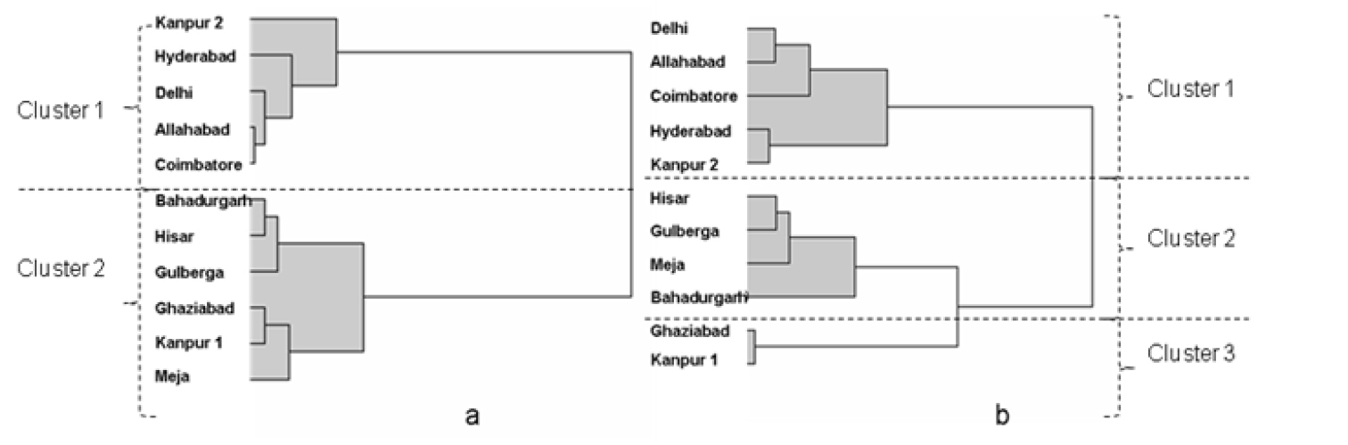
Dendograms from cluster analysis a) for the nine biometric measurements made on second stage juveniles of eleven populations of Heterodera cajani (see Table 2 for data) b) vulval cones of cysts of the same populations. (See Table 3 for data). The using the upper tail rule the best cut procedure indicated the highest number of significant cluster partitions was for a) 2 and for b) 3 with realized deviates and t- statistics respectively of a) 2.71 and 8.56 and b) 1.04 and 3.27.
AFLP banding from the two replicate DNA extracts was read for each population but no qualitative difference occurred between them. The eleven nematode populations were each tested with 64 pairs of primers to generate AFLP fingerprints. The number of amplification products ranged from 34 (primer pair +AAA, with +CTA) to 94 (+AAG with +CAG; Figure 2). A subset of 24 primer pair combinations of EcoR I and Mse I gave a good range of amplification products for all populations shown in Table 5. The fragments generated by the 24 selected primer pairs were recorded in a binary manner.
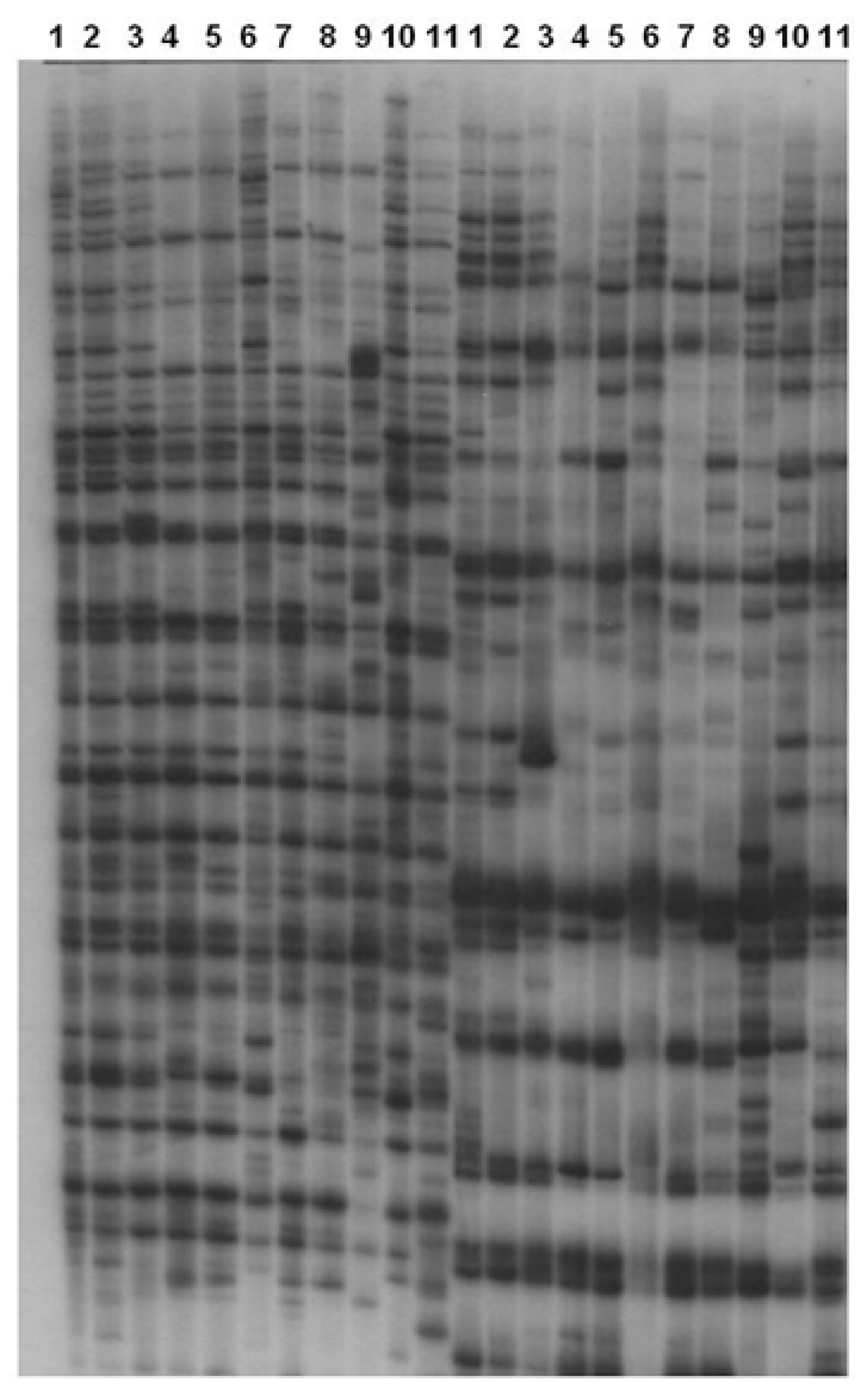
AFLP Autoradiogram of pigeon pea cyst nematode Heterodera cajani with EcoRI (+AAG) + MseI, (+CAG) and EcoRI (+AAA) + MseI (CTA). Lane 1 to 11: Heterodera cajani populations from Andhra Pradesh, Allahabad, Bahadurgarh, Coimbatore, Kanpur-1, Ghaziabad, Gilberga, Hisar, Delhi, Kanpur-2, andMeja.
Characterization of amplification products Obtained with 24 AFLP primer pairs used to analyze the genetic diversity of Heterodera cajani populations
| Primer EcoRI/MseI | Total number of fragments Obtained | |
|---|---|---|
| +AAA, | +CAA | 78 |
| +CAC | 71 | |
| +CAG* | 80 | |
| +CAT | 58 | |
| +CTA | 34 | |
| +CTC | 44 | |
| +AAC, | +CAA | 50 |
| +CAT | 73 | |
| +CTA* | 64 | |
| +CTC | 54 | |
| +AAG, | +CAA | 58 |
| +CAC* | 44 | |
| +CAG | 94 | |
| +CAT* | 73 | |
| +CTA | 69 | |
| +CTC | 69 | |
| +CTG | 59 | |
| +AAT, | +CAA | 44 |
| +CAC | 44 | |
| +CAG | 44 | |
| +CAT | 55 | |
| +CTA | 40 | |
| +CTC | 43 | |
Principal component analysis revealed that 44% and 33% of the full AFLP data set could be represented in three or two dimensions respectively (Table 6a). The corresponding values for a subset of four primers were 46% and 34% respectively (Table 6b). For both sets of data, four dimensions were required to represent just over 50% of the accumulative variation with 6-7 dimensions representing 75% of the variance. Therefore PC analysis was not used further for this data. As a consequence, all PC data for both morphometric and AFLP analyses are shown in tables rather than two or three-dimensional plots which cannot adequately represent the AFLP data.
Principal Component scores from cluster analysis for Heterodera cajani AFLP markers generated using 24 set of primer pairs
| Populations | Dimensions | |||||||||
|---|---|---|---|---|---|---|---|---|---|---|
| 1 | 2 | 3 | 4 | 5 | 6 | 7 | 8 | 9 | 10 | |
| Allahabad | 10.75 | -2.02 | 6.90 | -1.32 | -0.59 | 6.98 | -0.08 | -0.38 | 1.28 | 7.18 |
| Hyderabad | 11.45 | -2.46 | 8.08 | -5.01 | -2.66 | 10.63 | -0.37 | 0.90 | 1.20 | -6.59 |
| Bahadurgarh | 8.70 | 2.41 | 6.41 | 9.80 | 1.78 | 0.93 | 0.43 | 0.13 | 3.06 | -2.89 |
| Kanpur 1 | 4.72 | 3.56 | 0.29 | -1.84 | 3.38 | 5.30 | 11.10 | 5.63 | 0.42 | -1.44 |
| Gulberga | -0.32 | 2.36 | -0.44 | -2.92 | -3.53 | -0.31 | -5.14 | 7.86 | -0.46 | -1.25 |
| Ghaziabad | 10.46 | -3.95 | 4.00 | -6.50 | -2.35 | -4.86 | 3.96 | -1.58 | 6.47 | -1.80 |
| Hisar | -2.00 | 4.44 | 2.01 | 1.59 | -11.32 | 5.77 | 4.68 | -2.20 | 3.85 | -1.14 |
| Kanpur 2 | 6.14 | -8.70 | -4.41 | 0.83 | -1.59 | 2.48 | 2.27 | -4.31 | -5.39 | -2.22 |
| Delhi | -7.54 | -10.49 | 7.62 | -0.24 | 0.76 | 3.88 | 2.35 | 0.86 | 2.88 | -1.47 |
| Coimbatore | -2.15 | 7.30 | 0.19 | -4.26 | 5.36 | 5.08 | -0.96 | -5.41 | 3.62 | -1.86 |
| Meja | 6.42 | -7.56 | -6.62 | 1.40 | -0.24 | 7.61 | 0.22 | 2.01 | 9.07 | -1.44 |
| Accumulative % variance | 33 | 44 | 54 | 64 | 72 | 80 | 88 | 95 | 100 | |
Principal Component scores from cluster analysis for Heterodera cajani AFLP markers generated using 4 set of primer pairs
| Populations | Dimensions | |||||||||
|---|---|---|---|---|---|---|---|---|---|---|
| 1 | 2 | 3 | 4 | 5 | 6 | 7 | 8 | 9 | 10 | |
| Allahabad | -2.13 | -6.29 | -2.54 | 2.72 | -1.53 | -0.10 | 1.15 | -1.73 | 1.24 | 3.37 |
| Hyderabad | -2.75 | -6.23 | -3.55 | 3.22 | -4.36 | 0.19 | 1.98 | -1.87 | -0.20 | -1.93 |
| Bahadurgarh | -0.71 | -5.67 | -1.54 | 4.16 | 2.84 | -0.27 | 2.04 | 1.25 | 0.19 | -0.30 |
| Kanpur 1 | 0.22 | -1.70 | -0.43 | 3.20 | -2.07 | -0.48 | 2.14 | 0.11 | 5.04 | -0.60 |
| Gulberga | 0.44 | 0.45 | -0.41 | 0.33 | -0.50 | 2.24 | -0.66 | -1.48 | 0.11 | -0.08 |
| Ghaziabad | -1.65 | -5.22 | -0.53 | -2.26 | -2.03 | -2.59 | 1.03 | 1.85 | 0.67 | 0.08 |
| Hisar | -0.47 | -0.58 | -0.94 | 2.52 | -3.33 | 1.08 | 5.71 | 2.00 | -0.46 | 0.81 |
| Kanpur 2 | -6.42 | -2.00 | 1.84 | 1.59 | -0.06 | -1.79 | 3.72 | -2.39 | 0.56 | -0.04 |
| Delhi | -5.68 | 0.66 | -5.80 | 1.86 | -0.52 | -1.49 | 1.46 | 0.58 | 0.93 | 0.18 |
| Coimbatore | 2.48 | -0.85 | -1.13 | 4.17 | -1.92 | -4.12 | 1.21 | -0.82 | -0.21 | 0.23 |
| Meja | -5.94 | -2.27 | 1.33 | 4.95 | -2.88 | -0.48 | -0.79 | 1.78 | 0.35 | 0.23 |
| Accumulative % variance | 34 | 46 | 57 | 66 | 75 | 83 | 91 | 96 | 100 | |
Cluster analysis was used for the full AFLP set as described in the statistical methods and the best cut indicated three clusters (Figure 3a). The first cluster consisted of the Hyderabad, Allahabad, Ghaziabad and Bahadurgarh populations, the second included those from Delhi, Kanpur-2 and Meja while, the populations from Coimbatore, Kanpur 1, Gulberga and Hisar have been grouped as third cluster. Comparison of this dendogram with cluster trees provided by subsets of the 24 AFLP primer pairs suggested that the four highlighted in Table 5 with an asterisk provided similar dendograms to that generated by all the primer pairs (Figure 3b).
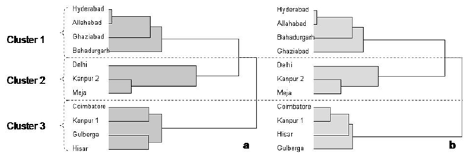
Dendograms from cluster analysis of Heterodera cajani a) for 1278 amplified restriction fragment digests using 24 primer pairs and b) the four primer pairs that suggest a similar dendogram to the full set. The using the upper tail rule the best cut procedure indicated the highest number of significant cluster partitions was 3 as in both cases with realised deviates and t statistics respectively of a) 1.47 and 4.66 and b) 1.59 and 5.04.
Mantel and partial Mantel tests did not detect a significant relationship between the matrix of geographical distances (see Figure 4 for a map showing locations of the 11 populations) and any of the three genetic distance matrices based on the data for J2s, cysts or AFLP (Table 7). Correlograms did not detect significant mantel r values or trends for the three sets of nematode data using five or more distance classes for the matrix of geographical distance. There was also no significant mantel correlation between the distance matrix for the full AFLP data set and for either set of morphological data.
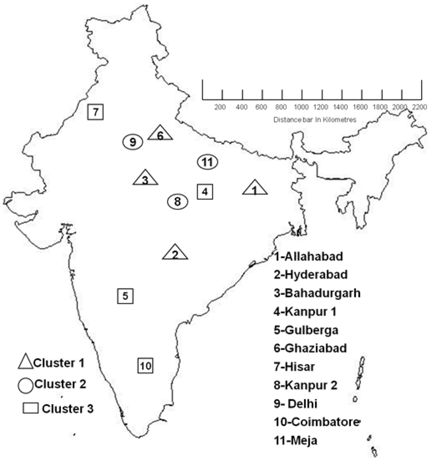
India Map showing distances of collected 11 Heterodera cajani populations with distances in (Kilometres)
Mantel tests for the relationships between the matrix of geographical distance and the three genetic distance matrices based on the data for J2s, cysts or AFLP.
| Type of Comparison with geographical matrix | Mantel test | Partial Mantel | ||
|---|---|---|---|---|
| r | t-value | r | t-value | |
| Biometric values on J2 | -0.08 | -0.61 | -0.06 | -0.43 |
| Biometric values on vulval cones | -0.20 | -1.43 | -0.18 | -1.24 |
| 24 AFLP primers | 0.13 | 0.78 | 0.12 | 0.73 |
| 4 AFLP primers | 0.03 | 0.14 | 0.02 | 0.12 |
| with 24 AFLP primer pairs distance matrix | ||||
| Biometric values on J2 | 0.09 | 0.63 | 0.10 | 0.68 |
| Biometric values on vulval cones | -0.05 | -0.33 | -0.06 | -0.44 |
Partial mantel tests were carried out a) for geographical distance among populations holding matrices not in the comparison constant with the 24 AFLP primer pair matrix being used when the biometric data was considered and b) for the correlations of the 24 AFLP primer pair genetic distance matrix with that for the two sets of biometic data holding that not in the comparison constant.
The two-morphometric sets of data and the AFLP approach all recognized significant clusters of populations within the set of eleven tested. All three approaches clustered the Allahabad and Hyderabad populations together and likewise the Gluberga and Hisar populations were similar as were Delhi and Kanpur 2 populations. Morphometrics disagree with AFLP for relationships between populations from Ghaziabad and Bahadurgarh, and for Coimbatore and Kanpur 1. Meja also was not placed with the same populations using both morphology and genetic approaches. This suggests that the morphometric approaches are of limited value for the analysis of intraspecific variation with in Heterodera cajani. The 11 populations used in this study have been analyzed before using RAPD analysis when a greater similarity between some of the populations than others was detected (
Previous work with Globodera pallida (a potato cyst nematode) using microsatellites in Peru has established high genetic similarly between individuals within a field. The limited active movement of J2s and males does not move them far in soil but tillage, either transport by surface water, running water and movement of infected potato tubers all contribute to a local homogeneity. Genetic similarity extends to neighboring fields and even those within a region which was defined as a range of about 35km for Globodera pallida in Peru (Piccard et al. 2004). This large passive dispersion is favoured inside an agronomic area where Globodera pallida has a continuous distribution and it is commonly at a high density (
Cluster analysis of both the AFLP and morphometric data revealed a similarity between populations belonging to different regions of India. Allahabad and Hyderabad cluster together for all approaches but they are about 2000 km apart as did Gulberga and Hisar which are 2200 km apart. Morphometric analysis on J2 means clustered Bahadurgarh and Meja populations together and Kanpur 1 population with that of Ghaziabad whereas the AFLP approach clustered these populations differently. AFLP analysis detected variation that was not evident in the morphological characters of J2s and vulval cones. Coimbatore is similar to populations in north India that are more than 2500 km from it (Figure 4). The two populations in closest proximity were those from Delhi and Ghaziabad. They are only 35 km apart but they did not cluster together with either AFLP or morphometric measurements. The variation we detected is not consistent with allopathic speciation over the large distances that prevail in India. It differs from the variation in Wucheria bancroftii in India which has been correlated with two geographically isolated and ancient introductions to this subcontinent (
Analysis of more Indian populations would be of value using the four primer sets that identify members of the three distinct AFLP clusters found in this work. The AFLP approach may correlate population differences with agricultural significant factors such as host range, virulence to pigeonpea resistance genes (
This is a first detailed study correlating morphological with molecular analysis of 11 populations of Heterodera cajani representing major pigeonpea growing areas in India. Morphometrics of Heterodera cajani though revealed some variation among the 11 populations but not as efficient as genetic analysis by AFLP. AFLP defined genetic variation had no relationship with geographical distance between populations. A sub-set of four AFLP primer sets clustered the 11 populations in the present study similarly to a larger group of 64 primer combinations. It may be useful for rapid, large scale characterization of additional populations. It could be applied to determine the extent of intraspecific variation among Indian populations of Heterodera cajani which occur on a range of legumes in the 20 agroclimatic zones and 60 sub regions in India (
We acknowledge Department of Science and Technology (DST) Govt of India, for providing financial support for this work. Thankful to Dr. K.V. Bhatt, NBPGR, New Delhi, Dr. K.K Kaushal, Dr. M. N Tripathi and Dr. A. K. Ganguly, Division of Nematology, IARI, New Delhi for providing microscope facilities and other basic nematology laboratory facilities to carry out the work.