


(C) 2012 R. Edward DeWalt. This is an open access article distributed under the terms of the Creative Commons Attribution License 3.0 (CC-BY), which permits unrestricted use, distribution, and reproduction in any medium, provided the original author and source are credited.
For reference, use of the paginated PDF or printed version of this article is recommended.
Ohio is an eastern USA state that historically was >70% covered in upland and mixed coniferous forest; about 60% of it glaciated by the Wisconsinan glacial episode. Its stonefly fauna has been studied in piecemeal fashion until now. The assemblage of Ohio stoneflies was assessed from over 4, 000 records accumulated from 18 institutions, new collections, and trusted literature sources. Species richness totaled 102 with estimators Chao2 and ICE Mean predicting 105.6 and 106.4, respectively. Singletons and doubletons totaled 18 species. All North American families were represented with Perlidae accounted for the highest number of species at 34. The family Peltoperlidae contributed a single species. Most species had univoltine–fast life cycles with the vast majority emerging in summer, although there was a significant component of winter stoneflies. Nine United States Geological Survey hierarchical drainage units level 6 (HUC6) were used to stratify specimen data. Species richness was significantly related to the number of unique HUC6 locations, but there was no relationship with HUC6 drainage area. A nonparametric multidimensional scaling analysis found that larger HUC6s in the western part of the state had similar assemblages with lower species richness that were found to align with more savanna and wetland habitat. Other drainages having richer assemblages were aligned with upland deciduous and mixed coniferous forests of the east and south where slopes were higher. The Ohio assemblage was most similar to the well–studied fauna of Indiana (88 spp.) and Kentucky (108 spp.), two neighboring states. Many rare species and several high quality stream reaches should be considered for greater protection.
Plecoptera, Stonefly, Biodiversity, Checklist, Ohio, North America
Regional biodiversity studies are of great importance for setting conservation priorities, in determining conservation status of species, and in examining factors that govern diversity (
Ohio is an eastern state of the USA with a total area of 105, 910 km2. It is bound on the south and east by the Ohio River and drained by 10 United States Geological Survey six digit scale Hydrologic Drainage Units (USDA 2009, HUC6s) (Fig. 1). The river and its tributaries have served as conduits for westward and northward migration from Kentucky, Pennsylvania, and West Virginia after the most recent glacial event cleared much of the fauna from the state. The Wisconsinan glaciation retreated 18, 000 years bp, leaving a highly modified landscape. Areas in the northwest two–thirds of the state were heavily glaciated, leaving till (west central), lake (NW), and drift (NE) plain landscapes. Southeast of this line is found the unglaciated Allegheny plateau, an area of deeply incised hills and valleys filled with glacial outwash. Pre-European settlement land cover in Ohio was dominated by upland forest (71%), wooded wetland (13.8%), and mixed deciduous and coniferous forest (Fig. 2), the overall similarity to the Appalachian forests diminishing rapidly westward. Ohio’s human population in 2010 was 11, 536, 504 (
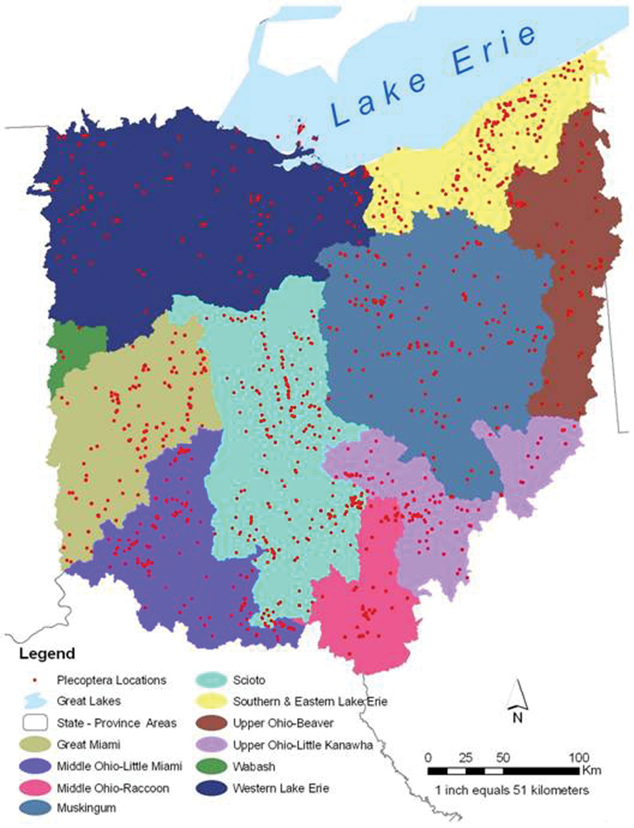
HUC6 drainages and point locations for Ohio Plecoptera collections.
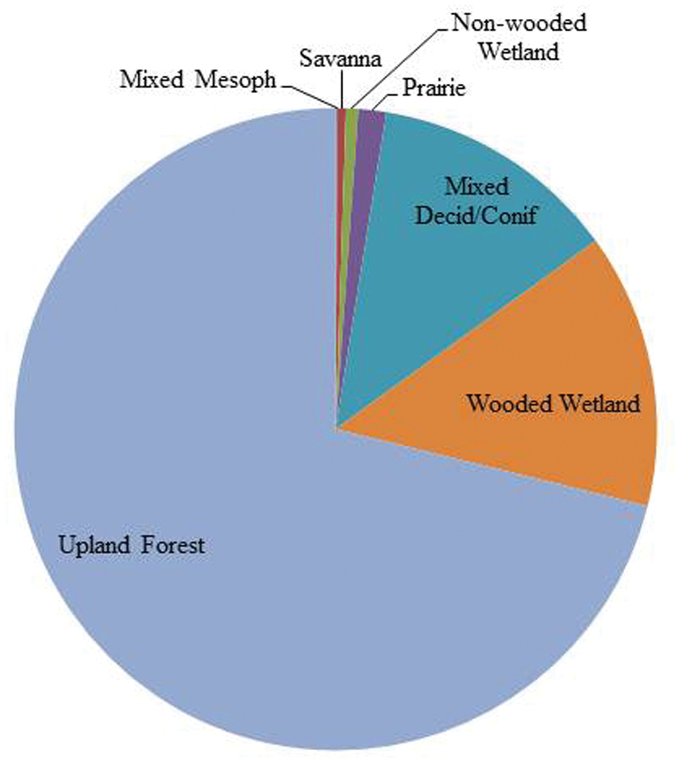
Pre-European settlement vegetation percentage cover for Ohio (from
Plecoptera (stoneflies) are known the world over as being environmentally sensitive (
Ohio’s stonefly fauna has been studied in a piecemeal fashion.
The coauthors have embarked on a study of the stonefly fauna of the Midwest, including distribution modeling of up to 160 species known from Illinois, Indiana, Michigan, Ohio, Ontario, and Wisconsin in order to reconstruct pre-European settlement range. Given that there has been no comprehensive assessment of the stonefly assemblage in Ohio we have elected to prepare one. This analysis is based on the accumulated specimen records from our own efforts, the efforts of colleagues over several decades, the examination of nearly 30, 000 specimens borrowed from regional museums, and reliable literature records. We ask several questions of these data:
• How many stonefly species inhabit Ohio?
• How completely has the fauna been sampled?
• How are functional niche traits distributed across the assemblage?
• Does drainage affiliation affect assemblage composition and species richness?
Methods Specimen RecordsSpecimens are the only resource where identifications may be verified, so the study was based on an abundance of specimens examined from 18 regional museums (Table 1). Pinned specimens were relaxed in a humid chamber and the terminalia cleared in 10% KOH. Cleared terminalia were acidified in dilute acetic acid, rinsed in water, and stored in glycerin under the specimens. Eggs were removed before clearing and rehydrated to view ultrastructural characters. Eggs were also stored in glycerin below the specimen. Adults in alcohol were dealt with similarly, the eggs and abdomens stored in shell vials inside the larger vial. Each specimen or series in a vial was associated with a database record using a paper catalog number. Label data and carefully scrutinized literature records were added to a local database. The raw data set is available as “Appendix 1 Raw Specimen data” in Excel Spreadsheet format. A glossary to Appendix 1 has also been provided as supplementary data.
Specimen origin, institutional coden, number of specimen records, and number of specimens examined.
| Institution | Coden | #Records | Specimens |
| Brigham Young University | BYU | 1167 | 18811 |
| B. P. Stark Collection | BPSC | 6 | 81 |
| Canadian National Collection | CNC | 46 | 252 |
| Cincinnati Museum of Natural History | CMNH | 2 | 2 |
| Cleveland Museum Natural History | CLEV | 66 | 171 |
| Field Museum Natural History, Chicago | FMNH | 13 | 40 |
| Illinois Natural History Survey | INHS | 639 | 2839 |
| Michigan State University | MSUC | 11 | 63 |
| Ohio Biological Survey | OBS | 573 | 2690 |
| Ohio Environmental Protection Agency | OEPA | 83 | 142 |
| Ohio Historical Society | OHSC | 17 | 17 |
| Ohio State University | OSU | 468 | 668 |
| Purdue University | PURC | 7 | 18 |
| R. Fred Kirchner Collection | RFKC | 164 | 857 |
| Royal Ontario Museum | ROME | 3 | 15 |
| Southern Illinois University Carbondale | SIUC | 1 | 5 |
| University of Michigan | UMMZ | 3 | 3 |
| Western Kentucky University | WKU | 170 | 873 |
| Literature | Author Year | 641 | 4940 |
| Total | 4, 080 | 32, 487 |
New specimens were collected using sweep nets, beating sheets, hand picking, and dipnetting throughout the state. Many nymphs were reared in Styrofoam cups or in a Frigid Units Living Stream at the University of Illinois. Illinois Natural History Survey (INHS) specimens collected after 2007 were preserved in 95% EtOH and stored in a –20C freezer for future molecular studies.
Locations for all specimens were georeferenced to the finest scale permitted by the label data. Coordinate precision for each record was marked as a radius about the location: from GPS = code 1(10 m); post–processed with small town or road crossing and stream name = code 2 (1, 000 m); town name only or large town with stream name = code 3(10, 000 m), county level record = code 4 (100, 000 m); state level record = code 5 (1, 000, 000) m. Only records with codes 1–3 were used for species accumulation curves and nonparametric multidimensional scaling (NMDS) analyses.
Data AnalysisHow many stonefly species inhabit Ohio and adequacy of sampling?These are complex questions that we answered in two ways. First, a list of species was tallied from all specimen data. All data were used for this purpose. Second, records with precision code 1–3 were used to estimate species richness using the program EstimateS v8.2 (
How are species traits distributed across the assemblage?
Ohio stoneflies. Stream widths inhabiting and functional niche traits. Width 1=seep, 2=1–2 m, 3=3–10 m, 4=10–30 m, 5=30–60 m, 6=>60 m, 7=Lake Erie. Voltinism 1, 2 or 3 yr; development 1=fast, 2=slow seasonal. Diapause 1=present, 2=absent. Dispersal Season W=winter, Sp=spring, Su=summer. Feeding O=omnivore, P=predator, S=shredder. Female Mobility L=low, M=moderate, H=high. Nymphal Growth=months of growth, Respiration 1=no gills, 2=with gills. Size at maturity 1=<9 mm, 2=9–16 mm, 3=>16 mm. Emergence Synchrony 1=>1 mo., 2=<1 mo. Thermal preference 1=coldwater, 2=coolwater, 3=warmwater. Active hyperlinks are embedded LSIDs linking to species pages in the Plecoptera Species File website (
| Species | Species Niche Traits | |||||||||||
|---|---|---|---|---|---|---|---|---|---|---|---|---|
| Stream Width | Voltinism | Development | Diapause | Dispersal Season | Feeding | Fem. Mobility | Nymphal Growth | Respiration | Size at Maturity | Synchrony | Thermal Pref. | |
| Capniidae | ||||||||||||
| Allocapnia forbesi Frison | 1–5 | 1 | 1 | 1 | W | S | L | 6 | 1 | 1 | 1 | 2 |
| Allocapnia frisoni Ross & Ricker | 2–3 | 1 | 1 | 1 | W | S | L | 6 | 1 | 1 | 1 | 2 |
| Allocapnia granulata Claassen | 3–6 | 1 | 1 | 1 | W | S | L | 6 | 1 | 1 | 1 | 3 |
| Allocapnia illinoensis Frison | 1–4 | 1 | 1 | 1 | W | S | L | 6 | 1 | 1 | 1 | 2 |
| Allocapnia indianae Ricker | 3–4 | 1 | 1 | 1 | W | S | L | 6 | 1 | 1 | 1 | 2 |
| Allocapnia mystica Frison | 2–4 | 1 | 1 | 1 | W | S | L | 6 | 1 | 1 | 1 | 2 |
| Allocapnia nivicola (Fitch) | 2–5 | 1 | 1 | 1 | W | S | L | 6 | 1 | 1 | 1 | 2 |
| Allocapnia ohioensis Ross & Ricker | 1–4 | 1 | 1 | 1 | W | S | L | 6 | 1 | 1 | 1 | 2 |
| Allocapnia pechumani Ross & Ricker | 3 | 1 | 1 | 1 | W | S | L | 6 | 1 | 1 | 1 | 2 |
| Allocapnia pygmaea( Burmeister) | 3 | 1 | 1 | 1 | W | S | L | 6 | 1 | 1 | 1 | 2 |
| Allocapnia recta (Claassen) | 2–5 | 1 | 1 | 1 | W | S | L | 6 | 1 | 1 | 1 | 2 |
| Allocapnia rickeri Frison | 2–5 | 1 | 1 | 1 | W | S | L | 6 | 1 | 1 | 1 | 2 |
| Allocapnia smithi Ross & Ricker | 2 | 1 | 1 | 1 | W | S | L | 6 | 1 | 1 | 1 | 2 |
| Allocapnia vivipara (Claassen) | 1–6 | 1 | 1 | 1 | W | S | L | 6 | 1 | 1 | 1 | 3 |
| Allocapnia zola Ricker | 3 | 1 | 1 | 1 | W | S | L | 6 | 1 | 1 | 1 | 2 |
| Paracapnia angulata Hanson | 1–4 | 1 | 2 | 2 | Sp | S | M | 11 | 1 | 1 | 2 | 1 |
| Leuctridae | ||||||||||||
| Leuctra alexanderi Hanson | 1–2 | 1 | 2 | 2 | Su | S | M | 11 | 1 | 1 | 1 | 2 |
| Leuctra duplicata Claassen | 3 | 1 | 2 | 2 | Su | S | M | 11 | 1 | 1 | 2 | 2 |
| Leuctra ferruginea (Walker) | 2–4 | 1 | 2 | 2 | Su | S | M | 11 | 1 | 1 | 2 | 2 |
| Leuctra rickeri James | 1–4 | 1 | 1 | 1 | Sp | S | M | 6 | 1 | 1 | 1 | 2 |
| Leuctra sibleyi Claassen | 2–4 | 1 | 1 | 1 | Sp | S | M | 6 | 1 | 1 | 1 | 2 |
| Leuctra tenella Provancher | 2 | 1 | 2 | 2 | Su | S | M | 11 | 1 | 1 | 2 | 2 |
| Leuctra tenuis (Pictet) | 2–4 | 1 | 1 | 2 | Su | S | M | 6 | 1 | 1 | 1 | 2 |
| Paraleuctra sara (Claassen) | 1–4 | 1 | 1 | 1 | Sp | S | M | 6 | 1 | 1 | 2 | 2 |
| Zealeuctra claasseni (Frison) | 2–3 | 1 | 1 | 1 | W | S | M | 6 | 1 | 1 | 1 | 2 |
| Zealeuctra fraxina Ricker & Ross | 2–3 | 1 | 1 | 1 | W | S | M | 6 | 1 | 1 | 1 | 2 |
| Nemouridae | ||||||||||||
| Amphinemura delosa (Ricker) | 1–5 | 1 | 1 | 1 | Sp | S | M | 6 | 2 | 1 | 1 | 2 |
| Amphinemura nigritta (Provancher) | 2–4 | 1 | 2 | 1 | Su | S | M | 9 | 2 | 1 | 1 | 1 |
| Amphinemura varshava (Ricker) | 1–6 | 1 | 1 | 1 | Sp | S | M | 6 | 2 | 1 | 1 | 2 |
| Nemoura trispinosa Claassen | 1–3 | 1 | 2 | 2 | Su | S | M | 11 | 1 | 1 | 1 | 1 |
| Ostrocerca albidipennis (Walker) | 2–3 | 1 | 1 | 1 | Sp | S | M | 6 | 1 | 1 | 1 | 1 |
| Ostrocerca truncata (Claassen) | 2–3 | 1 | 1 | 1 | Sp | S | M | 6 | 1 | 1 | 1 | 1 |
| Prostoia completa (Walker) | 2–3 | 1 | 1 | 1 | Sp | S | M | 6 | 1 | 1 | 2 | 2 |
| Prostoia similis (Hagen) | 2–3 | 1 | 1 | 1 | Sp | S | M | 6 | 1 | 1 | 2 | 2 |
| Soyedina vallicularia (Wu) | 1–3 | 1 | 1 | 1 | W | S | M | 11 | 1 | 1 | 1 | 1 |
| Taeniopterygidae | ||||||||||||
| Strophopteryx fasciata (Burmeister) | 3–6 | 1 | 1 | 1 | W | S | M | 6 | 1 | 2 | 1 | 2 |
| Taeniopteryx burksi Ricker & Ross | 2–6 | 1 | 1 | 1 | W | S | M | 6 | 2 | 2 | 1 | 3 |
| Taeniopteryx lita Frison | 6 | 1 | 1 | 1 | W | S | M | 6 | 2 | 2 | 1 | 3 |
| Taeniopteryx maura (Pictet) | 2–5 | 1 | 1 | 1 | W | S | M | 6 | 2 | 2 | 1 | 3 |
| Taeniopteryx metequi Ricker & Ross | 3–5 | 1 | 1 | 1 | W | S | M | 6 | 2 | 2 | 1 | 2 |
| Taeniopteryx nivalis Fitch | 3–5 | 1 | 1 | 1 | W | S | M | 6 | 2 | 2 | 1 | 2 |
| Taeniopteryx parvula Banks | 3–5 | 1 | 1 | 1 | W | S | M | 6 | 2 | 2 | 1 | 2 |
| Chloroperlidae | ||||||||||||
| Alloperla caudata Frison | 2–4 | 1 | 1 | 1 | Sp | P | M | 6 | 1 | 1 | 2 | 2 |
| Alloperla chloris Frison | 2–4 | 1 | 2 | 2 | Sp | P | M | 11 | 1 | 1 | 2 | 1 |
| Alloperla idei Ricker | 3 | 1 | 2 | 2 | Sp | P | M | 11 | 1 | 1 | 2 | 1 |
| Alloperla imbecilla (Say) | 2–3 | 1 | 2 | 2 | Sp | P | M | 11 | 1 | 1 | 2 | 1 |
| Alloperla neglecta Frison | 3 | 1 | 2 | 2 | Sp | P | M | 11 | 1 | 1 | 2 | 1 |
| Alloperla petasata Surdick | 2–3 | 1 | 1 | 2 | Sp | P | M | 6 | 1 | 1 | 2 | 2 |
| Alloperla usa Ricker | 2–4 | 1 | 2 | 2 | Sp | P | M | 11 | 1 | 1 | 2 | 1 |
| Haploperla brevis (Banks) | 1–3 | 1 | 1 | 1 | Sp | P | M | 6 | 1 | 1 | 2 | 2 |
| Sweltsa hoffmani Kondratieff & Kirchner | 1–5 | 1 | 2 | 2 | Sp | P | M | 11 | 1 | 1 | 2 | 1 |
| Sweltsa lateralis (Banks) | 3 | 1 | 2 | 2 | Sp | P | M | 11 | 1 | 1 | 2 | 1 |
| Perlidae | ||||||||||||
| Acroneuria abnormis (Newman) | 3–6 | 2 | 2 | 2 | Su | P | H | 23 | 2 | 3 | 2 | 2 |
| Acroneuria carolinensis (Banks) | 2–5 | 2 | 2 | 2 | Su | P | H | 23 | 2 | 3 | 2 | 2 |
| Acroneuria covelli Grubbs & Stark | 5 | 2 | 2 | 2 | Su | P | H | 23 | 2 | 3 | 2 | 2 |
| Acroneuria evoluta Klapálek | 4–6 | 2 | 2 | 2 | Su | P | H | 23 | 2 | 3 | 2 | 3 |
| Acroneuria filicis Frison | 2–6 | 2 | 2 | 2 | Su | P | H | 23 | 2 | 3 | 2 | 2 |
| Acroneuria frisoni Stark & Brown | 2–7 | 1 | 2 | 2 | Su | P | H | 11 | 2 | 3 | 2 | 2 |
| Acroneuria internata (Walker) | 4–6 | 2 | 2 | 2 | Su | P | H | 23 | 2 | 3 | 2 | 2 |
| Acroneuria kosztarabi Kondratieff & Kirchner | 3 | 2 | 2 | 2 | Su | P | H | 23 | 2 | 3 | 2 | 2 |
| Acroneuria lycorias (Newman) | 2 | 2 | 2 | 2 | Su | P | H | 23 | 2 | 3 | 2 | 2 |
| Acroneuria perplexa Frison | 3–6 | 2 | 2 | 2 | Su | P | H | 23 | 2 | 3 | 2 | 3 |
| Agnetina annulipes (Hagen) | 4 | 2 | 2 | 2 | Su | P | H | 23 | 2 | 3 | 2 | 2 |
| Agnetina capitata (Pictet) | 2–5 | 2 | 2 | 2 | Su | P | H | 23 | 2 | 3 | 2 | 2 |
| Agnetina flavescens (Walsh) | 2–6 | 2 | 2 | 2 | Su | P | H | 23 | 2 | 3 | 2 | 2 |
| Attaneuria ruralis (Hagen) | 4 | 2 | 2 | 2 | Su | P | H | 23 | 2 | 3 | 2 | 3 |
| Eccoptura xanthenes (Newman) | 2 | 2 | 2 | 2 | Su | P | H | 23 | 2 | 3 | 1 | 1 |
| Neoperla catharae Stark & Baumann | 3–5 | 1 | 2 | 2 | Su | P | H | 11 | 2 | 2 | 2 | 2 |
| Neoperla clymene (Newman) | 3–5 | 1 | 2 | 2 | Su | P | H | 11 | 2 | 2 | 2 | 3 |
| Neoperla coosa Stark & Smith | 3–5 | 1 | 2 | 2 | Su | P | H | 11 | 2 | 2 | 2 | 2 |
| Neoperla gaufini Stark & Baumann | 3–6 | 1 | 2 | 2 | Su | P | H | 11 | 2 | 2 | 2 | 2 |
| Neoperla mainensis Banks | 4–7 | 1 | 2 | 2 | Su | P | H | 11 | 2 | 2 | 2 | 3 |
| Neoperla occipitalis (Pictet) | 3–6 | 1 | 2 | 2 | Su | P | H | 11 | 2 | 2 | 2 | 2 |
| Neoperla robisoni Poulton & Stewart | 3–5 | 1 | 2 | 2 | Su | P | H | 11 | 2 | 2 | 2 | 2 |
| Neoperla stewarti Stark & Baumann | 2–6 | 1 | 2 | 2 | Su | P | H | 11 | 2 | 2 | 2 | 2 |
| Paragnetina media (Walker) | 3–5 | 2 | 2 | 2 | Su | P | H | 23 | 2 | 3 | 2 | 2 |
| Perlesta adena Stark | 2–6 | 1 | 1 | 1 | Su | P | H | 4 | 2 | 2 | 2 | 2 |
| Perlesta decipiens(Walsh) | 3–6 | 1 | 1 | 1 | Su | P | H | 4 | 2 | 2 | 2 | 3 |
| Perlesta golconda DeWalt & Stark | 3 | 1 | 1 | 1 | Su | P | H | 4 | 2 | 2 | 2 | 3 |
| Perlesta lagoi Stark | 3–6 | 1 | 1 | 1 | Su | P | H | 4 | 2 | 2 | 2 | 3 |
| Perlesta shubuta Stark | 3–6 | 1 | 1 | 1 | Su | P | H | 4 | 2 | 2 | 2 | 2 |
| Perlesta teaysia Kondratieff & Kirchner | 2–5 | 1 | 1 | 1 | Su | P | H | 4 | 2 | 2 | 2 | 2 |
| Perlesta xube Stark & Rhodes | 4 | 1 | 1 | 1 | Su | P | H | 4 | 2 | 2 | 2 | 2 |
| Perlesta sp. I–4 | 3-6 | 1 | 1 | 1 | Su | P | H | 4 | 2 | 2 | 2 | 2 |
| Perlinella drymo (Newman) | 3–5 | 1 | 1 | 1 | Su | P | H | 9 | 2 | 3 | 2 | 2 |
| Perlinella ephyre (Newman) | 3–6 | 1 | 1 | 1 | Su | P | H | 9 | 2 | 2 | 2 | 3 |
| Perlodidae | ||||||||||||
| Clioperla clio (Newman) | 1–5 | 1 | 1 | 1 | Sp | P | H | 9 | 1 | 2 | 2 | 2 |
| Cultus decisus decisus (Walker) | 2–3 | 1 | 2 | 2 | Sp | P | H | 11 | 1 | 2 | 2 | 1 |
| Diploperla robusta Stark & Gaufin | 1–5 | 1 | 1 | 1 | Sp | P | M | 6 | 1 | 2 | 2 | 2 |
| Isoperla bilineata (Say) | 3–6 | 1 | 1 | 1 | Su | P | H | 6 | 1 | 2 | 2 | 3 |
| Isoperla burksi Frison | 2 | 1 | 1 | 1 | Sp | P | M | 6 | 1 | 2 | 2 | 2 |
| Isoperla decepta Frison | 2–4 | 1 | 1 | 1 | Sp | O | M | 6 | 1 | 2 | 2 | 2 |
| Isoperla dicala Frison | 2 | 1 | 2 | 2 | Su | P | H | 11 | 1 | 2 | 2 | 2 |
| Isoperla holochlora (Klapálek) | 3 | 1 | 2 | 2 | Su | P | H | 11 | 1 | 2 | 2 | 1 |
| Isoperla montana (Banks) | 2–4 | 1 | 2 | 2 | Sp | P | M | 11 | 1 | 2 | 2 | 2 |
| Isoperla nana (Walsh) | 2–5 | 1 | 1 | 1 | Sp | P | M | 6 | 1 | 1 | 2 | 3 |
| Isoperla signata (Banks) | 2–4 | 1 | 2 | 2 | Su | P | H | 11 | 1 | 2 | 2 | 2 |
| Isoperla transmarina (Newman) | 2–4 | 1 | 2 | 2 | Sp | P | H | 11 | 1 | 2 | 2 | 2 |
| Malirekus cf. iroquois Stark & Szczytko | 3 | 1 | 2 | 2 | Su | P | H | 11 | 1 | 3 | 2 | 1 |
| Peltoperlidae | ||||||||||||
| Peltoperla arcuata Needham | 2–3 | 1 | 2 | 2 | Su | S | H | 11 | 2 | 2 | 2 | 1 |
| Pteronarcyidae | ||||||||||||
| Pteronarcys cf. biloba Newman | 3 | 3 | 1 | 1 | Su | S | H | 35 | 2 | 3 | 2 | 1 |
| Pteronarcys dorsata (Say) | 5–6 | 3 | 1 | 1 | Su | S | H | 35 | 2 | 3 | 2 | 2 |
Does drainage affiliation affect assemblage composition and species richness? HUC6 units were used to stratify the records (
The NMDS analysis was conducted using PC–ORD Ver. 5 (
Nine Ohio HUC6 drainages, number of unique locations, species richness and 16 environmental variables used in NMDS analysis. Pre-European settlement vegetation is percentage cover. PEMM = Portage Escarpment Mesophytic Forest, Forest_UL =Upland forest, Forest_MX = Mixed deciduous/coniferous forest, WL_NW = nonwooded wetland, WL_W = wooded wetland, RR_Mean = Relief Ratio mean.
| % Pre-European Settlement Vegetation | Elevation (m) | Relief Ratio | ||||||||||||||||
|---|---|---|---|---|---|---|---|---|---|---|---|---|---|---|---|---|---|---|
| USGS HUC6s |
Sites | Species Richness | DRAIN_km2X1000 | PEMM | PRAIRIE | FOREST_UL | FOREST_MX | SAVANNA | WL_NW | WL_W | ELEV_MEAN | ELEV_STD | ELEV_MAX | ELEV_MIN | ELEV_MEDIAN | RR_MEAN | RR_MEDIAN | SLOPE % |
| WL_Erie | 95 | 25 | 23.31 | 0.0 | 2.3 | 59.3 | 0.7 | 2.0 | 1.6 | 34.1 | 239 | 35.8 | 411 | 147 | 233 | 0.35 | 0.33 | 0.8 |
| SE_LErie | 133 | 65 | 8.25 | 1.2 | 0.1 | 68.8 | 24.0 | 0.0 | 1.0 | 4.9 | 285 | 53.9 | 420 | 173 | 285 | 0.45 | 0.45 | 2.2 |
| UOH_Bvr | 50 | 44 | 8.62 | 0.0 | 0.0 | 80.2 | 17.2 | 0.0 | 0.2 | 2.4 | 330 | 38.6 | 436 | 182 | 336 | 0.58 | 0.61 | 6.2 |
| UOH_LKan | 80 | 48 | 7.93 | 0.0 | 0.2 | 80.7 | 15.9 | 0.0 | 0.3 | 2.9 | 263 | 45.8 | 433 | 151 | 261 | 0.40 | 0.39 | 10.3 |
| Musk | 116 | 56 | 20.85 | 0.0 | 0.0 | 76.2 | 20.6 | 0.0 | 0.4 | 2.8 | 316 | 43.0 | 460 | 174 | 317 | 0.50 | 0.50 | 6.8 |
| Scioto | 201 | 71 | 16.87 | 0.0 | 3.9 | 69.9 | 12.1 | 0.0 | 0.3 | 13.7 | 283 | 43.2 | 454 | 142 | 289 | 0.45 | 0.47 | 3.9 |
| GrMiami | 109 | 34 | 10.70 | 0.0 | 1.3 | 79.4 | 5.1 | 0.0 | 0.4 | 13.8 | 299 | 44.7 | 469 | 138 | 306 | 0.49 | 0.51 | 1.9 |
| MOH_Rac | 39 | 35 | 5.06 | 0.0 | 0.0 | 84.9 | 10.0 | 0.0 | 0.0 | 5.1 | 233 | 34.1 | 363 | 136 | 234 | 0.43 | 0.43 | 9.8 |
| MOH_LMia | 119 | 57 | 9.37 | 0.0 | 1.8 | 60.8 | 16.4 | 0.0 | 0.0 | 21.0 | 269 | 45.5 | 404 | 131 | 275 | 0.50 | 0.53 | 4.6 |
A total of 4, 051 database records accounting for 32, 487 specimens were accumulated for this project (Table 1). The museum that contributed the most records was the Bean Museum at Brigham Young University, followed by the INHS Insect Collection. Cumulatively, these records produced an Ohio stonefly assemblage of at least 102 species (Table 2) from 942 unique locations (Fig. 1, Appendix 2).
Species richness estimators predicted slightly higher values (Fig. 3). The Chao2 estimator predicted 105.6 species with 95% confidence intervals (CI) ranging from 102.8 to 119.0 species. Another estimator, ICE Mean, produced a mean value of 106.4 (EstimateS does not provide CIs for this estimator). Many rare species were found. Singletons and doubletons accounted for 17.6% of all species (Fig. 4). Approximately 75% of all species were collected at fewer than 20 locations, while only three species were collected from over 100 locations: Allocapnia vivipara (Claassen) (223 sites), Perlesta cf. lagoi Stark (161 sites), and Acroneuria frisoni Stark & Brown (115 sites) (Fig. 5).
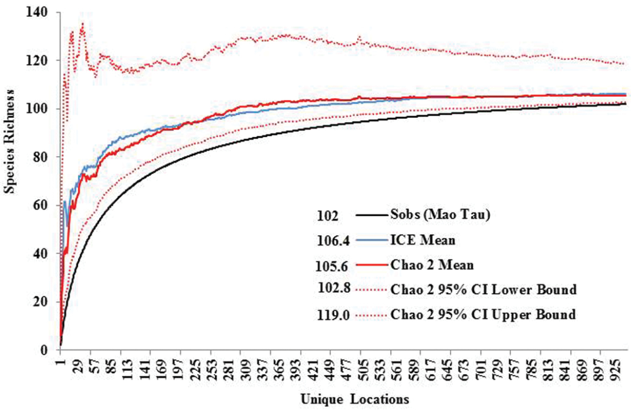
Ohio Plecoptera species richness, actual vs. predicted.
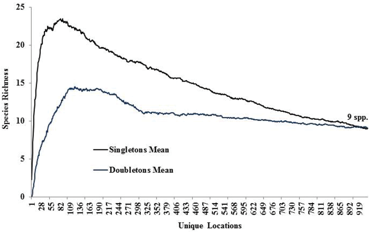
Singleton and doubleton species richness.
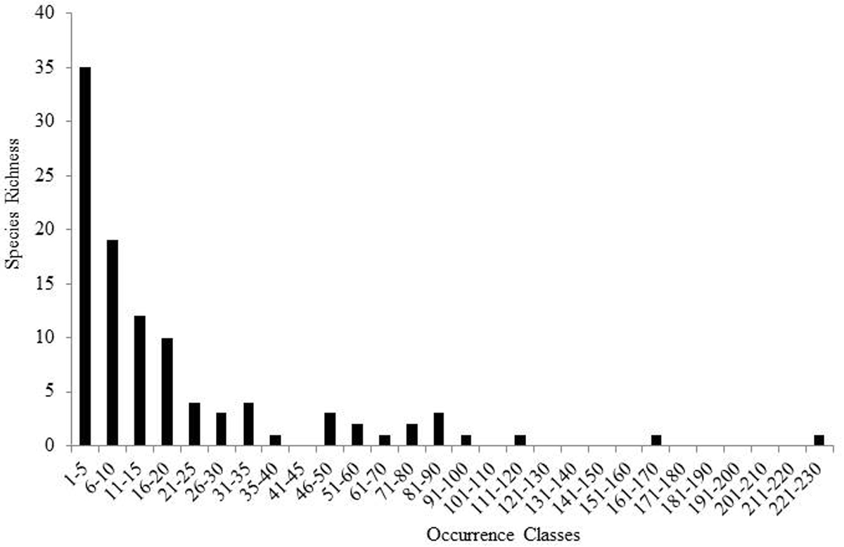
Species richness of Ohio Plecoptera in 5 increment occurrence classes.
The stonefly fauna of Ohio was represented by all nine families known to inhabit the North American continent (Fig. 6). Perlidae contributed the greatest number species (32.4%). Capniidae, one of the winter stonefly families, contributed 15.7% of all species found. Four other families contributed between 8.8% and 12.7% of the fauna. Roach stoneflies, Peltoperlidae, contributed a single species, Peltoperla arcuata Needham.
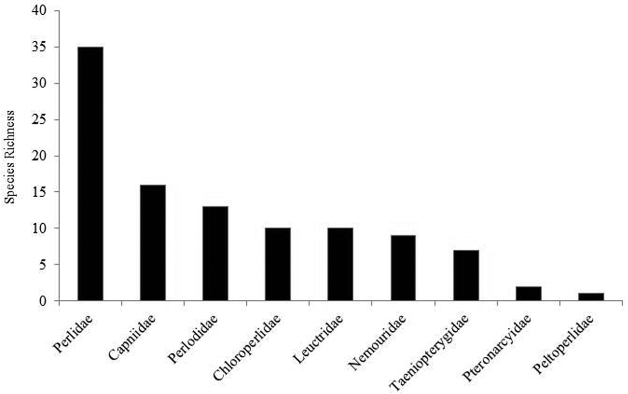
Species richness of Ohio Plecoptera families.
Stream size is often an important determinant of stonefly communities. This dataset demonstrated that most species inhabited a range of stream sizes (Table 2). There were several species relegated to small streams. Five species occurred only in streams that were 1 to 2 m across: Allocapnia smithi Ross & Ricker, Leuctra tenella Provancher, Eccoptura xanthenes (Newman), and Isoperla burksi Frison. Several others inhabited streams 3 to 10 m across: Allocapnia pechumani Ross & Ricker, Allocapnia zola Ricker, Leuctra duplicata Claassen, Acroneuria kosztarabi Kondratieff & Kirchner, Peltoperla arcuata Needham, and Malirekus cf. iroquois Stark & Szczytko. While some species were most frequently collected from large rivers, they could be taken in somewhat smaller streams as well. Only two species were confirmed to inhabit Lake Erie, from several locations around the Bass Islands: both perlids, Acroneuria frisoni and Neoperla mainensis Banks. Both species have been extirpated from Lake Erie, but Acroneuria frisoni is frequently collected throughout all but the northwestern corner of the state.
Distribution of Species TraitsThe vast majority of stonefly species inhabiting Ohio have single year life cycles; only 17 (16.7%) had multiyear life cycles (Table 4). Species with fast–seasonal cycles, those with nymphal growth periods that lasted 4-9 months, are slightly more frequently collected than slow seasonal (growth 11, 23, 35 mo. = direct development) species. Species with egg or nymphal diapause were also more frequently collected in Ohio than were non–diapausing species. Most species dispersed in the summer, a trait state that was not surprising given the number of perlid species found. Ohio did have quite a large proportion of so called “winter stoneflies”, species that emerge in winter that belong to the families Capniidae and Taeniopterygidae.
The number of months of nymphal growth had the largest number of trait states of all species trait categories. There were 9 species with an exceedingly short growth period of four months. These included all Perlesta species, a genus where females lay eggs in June and July and the eggs diapause until March. The most frequent growth period was 6 months, accounting for 40.8% of all species. Only a few species exhibited a nine month growing period, Perlinella, Clioperla clio (Newman), and Amphinemura nigritta (Provancher), while a total of 31 exhibited 11 month growth periods. Growth periods lasting 23 (Acroneuria, Agnetina, Attaneuria, Paragnetina) and 35 (Pteronarcys) mos. were also present.
Species traits distributions for the Ohio stonefly assemblage. Traits from Table 2.
| Volt. | Devel. | Diap. | Dispers. | Feed. | Mobil. | Grow. | Respir. | Size (mm) | Synch. (mo.) | Therm. | |||||||||||
| 1 | 85 | 1 | 57 | 1 | 56 | W | 25 | O | 1 | L | 15 | 4 | 8 | 1 | 56 | <9 | 46 | >1 | 36 | 1 | 19 |
| 2 | 15 | 2 | 45 | 2 | 46 | Sp | 28 | P | 56 | M | 42 | 6 | 42 | 2 | 46 | 9–16 | 35 | <1 | 66 | 2 | 67 |
| 3 | 2 | Su | 49 | S | 45 | H | 45 | 9 | 4 | >16 | 21 | 3 | 16 | ||||||||
| 11 | 31 | ||||||||||||||||||||
| 23 | 15 | ||||||||||||||||||||
| 35 | 2 | ||||||||||||||||||||
More research on the feeding of Plecoptera nymphs and adults is necessary to effectively use functional feeding group designations for ecological research. The study of gut enzymatic activity (
Female mobility is an important trait that confers ability to colonize and recolonize after local extinction. The vast majority of species exhibited medium to high female mobility. Low female dispersal ability was exhibited by 14.6% of Ohio species. Low mobility is a complex character state that is exhibited mostly by winter emerging species that emigrate by crawling, skating (wings held up to breeze and skating on tarsi), or floating on logs or ice floes.
The presence or absence of gills is often thought of as indicative of a species’ ability to tolerate warmer waters and lower oxygen concentrations. No formal analysis has been conducted of the association of gilled stoneflies with water temperature preference, but informal studies in Europe indicate that many gilled species inhabit mountainous areas with cold and cool water temperatures (M. Tierno de Figueroa pers. comm.). In eastern North America there are over 50 species of perlids (Attaneuria, Perlesta, Perlinella, Neoperla, Acroneuria, Agnetina, and Paragnetina) that tolerate warmer streams and often dominate the stonefly assemblage at low elevation.
The majority of Ohio species (54.9%) did not have gills (some Perlodidae with submental gills were counted as gill-less). Most of these species lived in cool and coldwater streams or lived in streams as nymphs only during the colder times of the year (e.g., they have diapause that restricts nymphs to winter or spring season). A total of 45.1% of species used gills. The vast majority of these were species in the family Perlidae.
Size at maturity is a trait that has direct bearing on risk to survival. Larger species are usually longer lived and exposed to risks for a longer period of time and may make more attractive prey items than some smaller species. Small species (<9 mm total length) were much more frequent in the list than large species (>16 mm). Smaller species are more likely to have short growth periods and diapause. They are also more likely to have fast cycles and disperse in the winter and spring than larger species.
Species with synchronous (<1 month) emergence periods were more frequent in Ohio than asynchronous (>1 month) species. Winter emerging species tend to have less synchronous emergence periods due to fluctuating winter temperatures from freezing and thawing. Those that emerge in spring and summer have sharper seasonal cues that lead to nymphal development being more synchronous, leading to emergence of adults over a shorter period of time. Spring and summer emerging species were three times more frequent in Ohio than winter-emerging ones; hence, the great disparity in synchronous over asynchronous emergence is easily understood.
Thermal requirements are not well understood in stoneflies or other aquatic insects and the terms coldwater, coolwater, and warmwater are relative when it comes to defining a temperature requirement. Trait state assignment here is based more on professional experience than for any other set of traits. Coldwater species contribute only 18.6% to the total number of species found in OH. Most of Ohio is or was heavily wooded, a feature usually related to coolwater conditions. This is by far the most frequent thermal tolerance state for stoneflies in Ohio. Another 15.7% of species can truly be categorized as warmwater species. This would include several perlid species.
Does drainage affiliation affect assemblage composition and species richness? Two measures of sample intensity across the nine HUC6 drainages demonstrated that three HUC6s were most heavily sampled: Southern and Eastern Lake Erie, Scioto, and Middle Ohio and Little Miami drainages (Fig. 7A). The two largest drainages, Western Lake Erie and Muskingum appeared to be somewhat under-sampled compared to other drainages. Across all drainages, species richness was significantly related to the number of unique locations sampled (R2=0.42, p=0.03, n=9, Fig. 7B). Western Lake Erie and Great Miami drainages had lower than predicted species richness. These are the western-most drainages in the state with a landscape composed of flatter till and lake plains, possibly accounting for lower species richness. There was no significant relationship between species richness and drainage area (R2=0.0, p=0.87, n=9) or the square root of drainage area (R2=0.0, p=0.97, n=9).
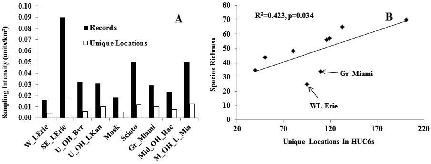
A–B Sampling intensity, drainage area, unique locations, and species richness relationships for HUC6 drainages A Sampling intensity for HUC6 drainages B Species richness vs. number of unique locations in HUC6 drainage areas.
Randomization tests in the NMDS analysis recommended a three dimensional solution. An overall stress value for the three dimensional analysis was low at 1.53. A plot of Axis 1 vs Axis 3 separated the communities of Ohio stoneflies best (Fig. 8). The western–most HUC6 drainages (Western Lake Erie and Great Miami) were separated from all other assemblages by being strongly associated with wetland and savanna pre-European settlement land covers. There was a lesser association with large total area as well. These two drainages supported the lowest species richness. Centrally located in the plot were five HUC6 communities that associated with low percentage wetland and savanna coverage and with smaller drainage sizes. These drainages had much richer stonefly communities and an association with upland hardwoods. Two other HUC6 assemblages (Upper Ohio Little Kanawha and Middle Ohio Raccoon) were separated from the others by being associated with a high percentage of mixed deciduous/coniferous forest and high percentage slope.
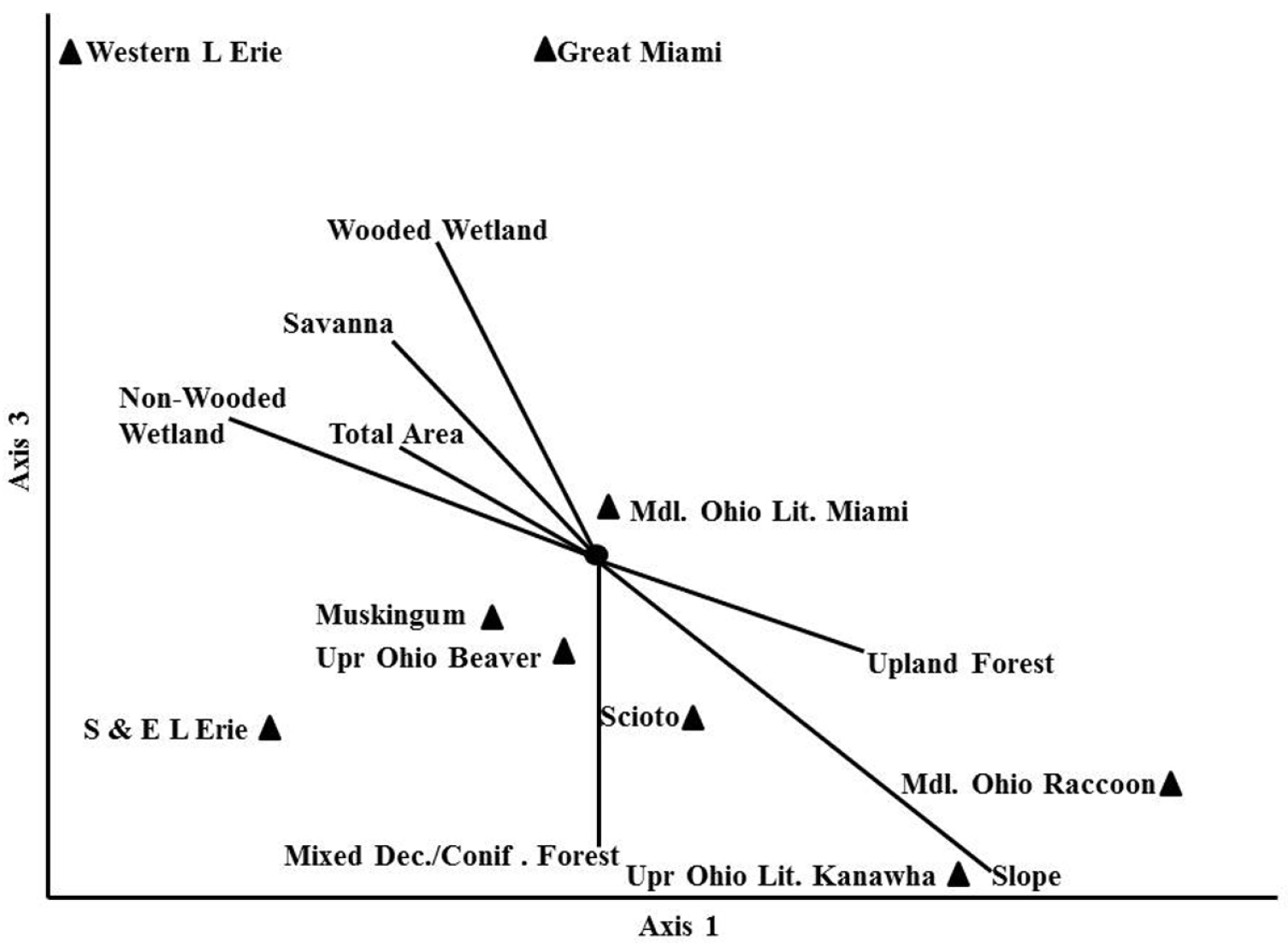
Non–parametric Multi–Dimensional Scaling of Ohio Plecoptera assemblages associated with HUC6 drainages. Axis 1 vs Axis 3.
Ohio is a state that has its eastern flank in the Allegheny Plateau, an extension of the Appalachian Mountains. Ohio’s western flank is mostly till plain resulting from the Wisconsinan glaciation. The stonefly fauna found in the state is a mixture of species requiring cooler waters and deep forest and those that have evolved with warmwater streams and even intermittency of flow. The number of species occurring in Ohio is indicative of being between these two extremes. Ohio supports at least 102 species, maybe as high as 119 (e.g., Chao 2 upper 95 percentile) (Fig. 4). Pennsylvania to the east supports 39.2% more species than Ohio, with West Virginia having 36.3% more species. It appears that a continuous drop of species occurs westward and northward from Ohio (Fig. 9). The northward decline of species occurs as species usually inhabiting unglaciated terrain drop out. Sørensen’s Index of Similarity suggested that Kentucky and Indiana assemblages have the greatest similarity with the Ohio assemblage, rather than the more mountainous states of Pennsylvania and West Virginia (Table 5). The lowest similarities were observed with more recently glaciated Michigan, Ontario, and Wisconsin.
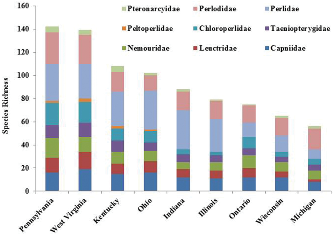
Comparison of Ohio Plecoptera assemblage with Midwest states/provinces.
Sørensen Index of Similarity between Plecoptera assemblages for nearby states/provinces in relation to Ohio. Codes are IL=Illinois, IN=Indiana, MI=Michigan, OH=Ohio, ON=Ontario, WI=Wisconsin, PA=Pennsylsvania, WV=West Virginia, and KY=Kentucky.
| IL | IN | MI | OH | ON | WI | PA | WV | KY | |
| IL | 0 | ||||||||
| IN | 0.814 | 0 | |||||||
| MI | 0.444 | 0.417 | 0 | ||||||
| OH | 0.659 | 0.743 | 0.415 | 0 | |||||
| ON | 0.416 | 0.429 | 0.656 | 0.551 | 0 | ||||
| WI | 0.569 | 0.523 | 0.744 | 0.548 | 0.686 | 0 | |||
| PA | 0.425 | 0.470 | 0.394 | 0.629 | 0.535 | 0.512 | 0 | ||
| WV | 0.440 | 0.485 | 0.349 | 0.628 | 0.467 | 0.461 | 0.826 | 0 | |
| KY | 0.588 | 0.684 | 0.354 | 0.749 | 0.437 | 0.474 | 0.648 | 0.721 | 0 |
Ohio had 18 species that were collected from just one or two locations, 17.6% of all species found. A discussion for a limited number of these species is presented below to identify for state, federal, and non–profit conservation organizations that these species, and the streams in which they reside, should be considered for protected status. Some streams are already in the public trust.
Allocapnia indianae Ricker. A large series was collected by W. E.
Allocapnia smithi Ross & Ricker. This species was taken from a single location in Warren Co., 10 km ESE Lebanon, Randall Run, Fort Ancient State Memorial, 39.40951, -84.09039, 12 February 1966, H. B. Cunningham. This species is known from scattered locations in unglaciated sections of Alabama, Illinois, Indiana, Kentucky, and Ohio (
Leuctra duplicata Claassen. This species was taken from two small streams adjacent to each other in Ashtabula Co.: 4.5 km NNW Hartsgrove at Callahan Rd., Crooked Creek, 41.64210, -80.97250, 3 June 1997, R. W. Baumann & B. C. Kondratieff, 7 males, 9 females; same location, 2 June 1989, R. W. Baumann & R. F. Kirchner, 2 M; Callahan Road, spring fed tributary Crooked Creek, 41.64245, -80.97374, 2 June 1989, R. W. Baumann & R. F. Kirchner, 42 males, 28 females. Crooked Creek is a darkly stained, 3–m wide stream that holds other coolwater species such as Acroneuria carolinensis (Banks), Isoperla cf. montana (Banks), Soyedina vallicularia (Wu), Paracapnia angulata Hanson, Allocapnia rickeri Frisonр and Taeniopteryx metequi Ricker & Ross. This species is known from much of northeastern North America, but Ohio is the furthest west it has been collected (
Alloperla idei Ricker. This species is represented by two records in the Allegheny Plateau region of SE OH. Lawrence Co., 17 km SSE Oak Hill, Buffalo Creek, Wayne National Forest, 38.74598, -82.54445, 27 May 2010, S. A. Grubbs, 3 males, 9 Females; Pickaway Co. Laurelville, Tributary Laurel Run, 39.47390, -82.74263. 23 May 1953, [A. R. Gaufin], 2 males. This species occurs throughout much of eastern Canada and the eastern USA (
Alloperla neglecta Frison. This species was collected as a single adult male from Lake Co., at Paine Road, Leroy Township, Paine Creek, Paine Falls Metropolitan Park, 41.71669, -81.14356, 31 May 1975, M. K. Tkac.
Sweltsa lateralis (Banks). Several adults were collected from Mahoning Co., Lowellville, Grays Run, 41.04353, -80.53957, May 1985, D. W. Fishbeck. This Gray’s Run was recorded as supporting several other species of Appalachian Mountains or coldwater habitat.
Peltoperla arcuata Needham. This species was once thought to be exceedingly rare in Ohio, but it has been located in four counties now in 1 to 2–m wide coldwater, ravine streams, usually associated with mixed deciduous and coniferous (hemlock and white pine) forest. This is the only representative of the family Peltoperlidae to inhabit Ohio. Loss of this species would remove an entire family of stoneflies from the state. Locations include: Ashland Co., Tributary to Hog Hollow Creek, Big Lyon Falls Creek, Little Lyon Falls Creek, Tributary Clear Fork Mohican River (Hemlock Grove CG), all in Mohican State Park; Knox Co., Tributary Mohican River at Greer; Mahoning Co., Gray’s Run at Lowellville; Muskingum Co., Seep Tributary Wills Creek. The species is distributed over several eastern states and the Canadian province of Quebec (
Isoperla burksi Frison. Three nymphs were collected from Scioto Co., Mackletree Run, 12 km SSW West Portsmouth, Shawnee State Forest. 38.7236, -83.1821, 14 April 2006, R. E. DeWalt, S. K. Ferguson, R. F. Kirchner. This species has been collected from the Ozark Mountains to New Jersey, mostly in unglaciated habitats. Mackletree Run is a stream that typifies semi–permanent streams in unglaciated southern Ohio.
Malirekus cf. iroquois Stark & Szczytko. We have seen two nymphs from a single location in Monroe Co., Tributary Stillhouse Run, 39.78146, -80.85288. M. Leuhrs.
Pteronarcys cf. biloba Newman. Nymphs with lateral extensions of the abdominal terga have been known from Ohio since Tkac’s (1979) dissertation, but no adults have been collected and the record was not published.
Several streams across the state are exceedingly rich in species and have been well sampled. A tributary of the East Branch of the Chagrin River in Stebbins Gulch of Holden Arboretum (Geauga Co.) produced 28 species including several coldwater species. A tributary of the East Fork Queer Creek at Ash Cave (Hocking Co.) has produced 23 species. The Olentangy River near Columbus (Franklin Co.) has produced 17 species historically. Upstream of the city near Highbank Metropark a diverse assemblage still persists, although it may not hold the full complement of species once found in the river. The Clear Fork of the Mohican River within the ravine area of Mohican State Park (Ashland Co.) has produced 14 species and probably still supports most of them. Big Lyons Falls Creek, also in Mohican State Park; a tributary of the North Fork Little Beaver River, 5 km S Negley, in Columbiana Co.; and Mill Creek at Doty Road (Lake Co.) all produced 13 species. Gray’s Run at Lowellville (Mahoning Co.) produced a total of 12 species, many of which were Appalachian coldwater species. Most of these locations are protected by public or private means. These, and several others too numerous to list here, are important for protecting the lotic diversity of aquatic organisms in the Ohio.
HUC6 DrainagesHUC6 drainages explain some of the variation in stonefly communities across Ohio (Fig. 8). However, the stress value was relatively low for this analysis, suggesting that there may be better stratification systems and variables to explain Ohio species richness patterns. Additional classification systems that could be tested in future analyses include U. S. Environmental Protection Agency level III ecoregions and the Nature Conservancy’s Ecological Drainage Units.
The data suggested that smaller drainages of the eastern and southern part of the state followed a pattern of increasing richness with drainage area, but that the largest drainage did not (Fig. 7B). Western Lake Erie was under-sampled in relation to its area (Fig. 7A, B). However, this is not to say that the species richness in the drainage was suspiciously low. The Western Lake Erie assemblage was defined by wetland categories and large drainage area (Fig. 8). This basin has low topographic relief and fine substrates left behind by large glacial lakes. The low species richness there was most likely a function of the flatter landscape, low current velocity, and finer substrates. The Great Miami drainage just to the south of Western Lake Erie also had relatively low species richness. It too was defined by similar environmental conditions as Western Lake Erie, however, its southern end contains one coldwater stream (Mad River) and fast flowing reaches, which enhanced its species richness over that of Western Lake Erie. Indeed, the two drainages had a 61% Sørensen quotient of similarity. The Great Miami basin supported such cool- and coldwater species as Agnetina capitata (Pictet), Paragnetina media (Walker), Leuctra tenuis (Pictet), Nemoura trispinosa Claassenр and Soyedina vallicularia (Wu). Several species that require faster flowing, wooded streams were also found in the Great Miami and not the Western Lake Erie drainage.
Some of the most species rich HUC6 assemblages were located in a band of upland forest and higher gradient streams that straddled drift plain and unglaciated terrain from Cincinnati to Ashtabula. These assemblages were dominated by widespread species that typically inhabit cool and warmwater streams. There was also a small component of coldwater Appalachian fauna including species of Ostrocerca, Amphinemura nigritta, Cultus decisus decisus, Malirekus cf. iroquois, Pteronarcys cf. biloba, Amphinemura neglecta, Alloperla lateralis, Alloperla idei, and Allocapnia pechumani, among others. These species have found coldwater habitat in ravine streams of Southern and Eastern Lake Erie, Upper Ohio and Beaver, Scioto, and Muskingum drainages.
Two other drainages, the Upper Ohio Little Kanawha and the Middle Ohio Raccoon, had assemblages that were defined by mixed deciduous and coniferous forests and higher slope values in southern, unglaciated Ohio. These are relatively small drainages with short streams, many of which become intermittent in the summer. Consequently, many species with egg or nymphal diapause are found here. This trend also occurs in southern Illinois and Indiana (
The Plecoptera assemblage presented herein is largely of pre-European settlement nature from records spanning the late 1880s to present. Some changes are likely to have occurred in Ohio, just as they did in IL (
Acroneuria abnormis (Newman). Once found in moderately large to large rivers throughout the state, it is now only known from recent records in the Grand River (Lake Co.), Clear Fork Mohican River (Ashland Co.), and Ohio River (Clermont Co.).
Acroneuria frisoni Stark & Baumann. This species was found at 115 unique locations across the state, with many being from recent years. Many historical records of adults and nymphs were found for the Bass Islands in the Western Basin of Lake Erie. Unfortunately, of the 94 records from the islands, the most recent was for 1961. It has been extirpated from Lake Erie.
Acroneuria filicis Frison. It once inhabited several moderately sized drainages in the eastern half of the state. The only recent records are from the Grand River (Lake Co.), West Fork River (Brown Co.), and Ohio Brush Creek (Scioto Co.).
Acroneuria perplexa Frison. This species has been lost from moderately large and large rivers in the eastern half of Ohio. No records are available for over 50 years. It is probably extirpated from Ohio.
Acroneuria evoluta Klapálek: There is a single historical record from 1936 from Black Lick Creek near Columbus (Franklin Co.). It is probably extirpated from Ohio.
Attaneuria ruralis (Hagen). A male and female of this large species were collected from Columbus (Franklin Co.), either from the Olentangy or Scioto rivers, in 1925. It is probably extirpated from Ohio.
Neoperla mainensis Banks. This species was historically collected from Columbus (Franklin Co.), either from the Scioto or Olentangy rivers; the Clear Fork of the Mohican (Ashland Co.), and South Bass Island (Ottawa Co.) area of Lake Erie. It is probably extirpated from the state with none of the 38 records being more recent than 1922.
ConclusionsA large dataset from 18 regional museums, new collecting, and trusted literature sources demonstrated that the Plecoptera assemblage of Ohio is rich with at least 102 species. All nine North American families were represented with Perlidae contributing 33% of all species (Fig. 6).
Ohio species are mostly univoltine-fast with egg or nymphal diapause and the largest proportion of them are summer emerging (Table 4). Nymphs are predominantly predatory, but a large number of species that shred conditioned leaves and wood were also present. The majority of species inhabited cool, forest-covered streams. The state has significant Appalachian elements, mostly within the ravine streams of central and eastern drainages associated with upland forests and mixed deciduous and coniferous forest habitats (Fig. 8). Despite this, the fauna of Ohio is most closely aligned with Indiana and Kentucky assemblages (Table 5).
It appears that Ohio has been well sampled; species estimators (Chao2 and ICE Mean) suggested that 3 or 4 more species could be found. Given that neighboring Pennsylvania and West Virginia have 142 and 139 species, respectively, it is likely that species shared with them will eventually be found in Ohio (Fig. 9). It is highly probably that these additional species will be located in ravine streams in eastern and southern Ohio.
A great number of species in Ohio were rare, being known from only 1–5 locations (Figs. 4 and 5). Many of these are candidates for protection, as are several stream reaches that support high numbers of species or assemblages that are rare. In addition, it appears that several species have experienced local or statewide extirpations. These have mostly been of univoltine and semivoltine species whose eggs hatch directly. This is consistent with losses reported for IL (
This paper lays a foundation for planned future work, including natural range modeling of species within the larger framework of the Midwest USA and Canada. This will allow our research team to reconstruct pre-European settlement ranges for most species in the region. We are also focusing considerable effort to use these baseline distributions against which to measure climate related changes in distribution by modifying climate variables in light of predicted CO2 emissions scenarios.
The authors thank several individuals for loan of specimens: Bill Stark (BPSC), Richard Baumann and Shawn Clark (BYU), Ian Smith (CNC), Gregory Dahlem (CINC), Joe Keiper (formerly CMNH), Daniel Summers (FMNH), Gary Parsons (MSUC), Brian Armitage (OBS), Michael Bolton (OEPA), Bob Glotzhober (OHSC), Norm Johnson (OSUC), Arwin Provonsha (PERC), Fred Kirchner (RFKC), Antonia Guidotti (ROM), Jay McPherson (SIUC), and Mark O’Brien (UMC). We also wish to thank Donald W. Webb for his contributions at the beginning of this effort. This work was partially supported by the National Science Foundation DEB 09–18805 ARRA.
Raw data and data matrices. (doi: 10.3897/zookeys.178.2616.app1) File format: MS Excel spreadsheet (xls).
Explanation note: Appendices include an Excel spreadsheet with all data used in analyses for this article: "Appendix1 Raw Specimen Data", "Glossary Appendix 1", "Appendix 2 OH Unique Locations", "Appendix 3 spp. Location Matrix", and "Appendix 4 spp. vs HUC6s".